[ REGULAR ]

Journal of the Korean Society for Precision Engineering - Vol. 36, No. 8, pp.683-690

ISSN: 1225-9071 (Print) 2287-8769 (Online)

Print publication date 01 Aug 2019

Received 26 Mar 2019 Revised 14 Jun 2019 Accepted 04 Jul 2019

DOI: https://doi.org/10.7736/KSPE.2019.36.8.683

Deep Regression for Precise Geometric Dimension Measurement

Thang Duong Nhat¹ ; Binh Nguyen Duc² ; Phuong Le Khac² ; Ngoc Tu Nguyen³ ; Mai Nguyen Thi Phuong⁴^{, #}

1Artificial Intelligence team, NAL Vietnam JSC, Hanoi, Vietnam
2Center for Training of Excellent Students, Hanoi University of Science and Technology, 1 Dai Co Viet Road, Hanoi, Vietnam
3National Canter for Technological Progress, Hanoi, Vietnam
4Department of Precision Mechanical and Optical Engineering, Hanoi University of Science and Technology, 1 Dai Co Viet Road, Hanoi, Vietnam

Correspondence to: ^#E-mail: mai.nguyenthiphuong@hust.edu.vn, TEL: +84-913345972

Copyright © The Korean Society for Precision Engineering
This is an Open-Access article distributed under the terms of the Creative Commons Attribution Non-Commercial License (http://creativecommons.org/licenses/by-nc/3.0) which permits unrestricted non-commercial use, distribution, and reproduction in any medium, provided the original work is properly cited.

Abstract

A planar-dimensions vision measurement method is proposed by developing a Neural Network to measure real-world distance between any two points on the plane. The system leveraging Neural Network ability to search in the solution space is a highly non-linear model that could map points’ location on the pixel plane of image(s) with the actual distance between them considering the non-uniform geometric distortion in captured images caused by the entocentric lens in a common camera. The method was tested with a printed calibration chessboard, placed in different locations on the plane, with measured distance between tested points. Experimental results show the proposed method’s mean absolute error is 1.24 × 10^-2 mm and standard deviation is 1.63 × 10^-3 mm, tested with 10-folds cross-validation method.

Keywords:

Deep learning, Planar-dimension measurement, Geometric distortion

1. Introduction

Geometric measurement is being used widely in the industry.^1-3 Since a planar-dimensions measurement system has the advantage of lower in cost, more precise (since there is no matching image cross camera process), there have been a number of applications in the field of industrial measurement.^4,5 Still, there exist some disadvantages in the use of the general optical instrument in 2D measurement such as long measuring time, personnel's subjective error and hard to integrate the system into a fully automatic measuring process. Thus, the introduction of computer vision technology in geometric measurement achieved huge success with its non-contact, fast processing speed, robust and high precision characteristic.

Using Computer Vision (CV), several measuring methods and improvements have been proposed.^6-8 Unlike the traditional methods, the CV based methods suffered from two major error sources: measurement errors from the software and systematic errors from the hardware. The measurement errors are mostly generated when an algorithm is used to schematized edge points or to determine the sub-pixel location of key features. Systematic errors came from image distortions (due to lens aberrations and misalignment of optical elements⁹), digitization error and others. Not just the common camera with entocentric lens, even those with high-quality telecentric lens cause non-uniform image distortion, corrupt the sub-pixel detection algorithms, thus, reduce the precision in measurement. With increasingly higher precision requirement, multiple techniques.^10-12 have been developed to use in measuring process to mitigate the effect of image distortion, and they have been successfully applied for 3D measurement.

In general, using a uniform model of image distortions in the camera calibration process proves its limited effectiveness.^13,14 This calibration procedure often used the Brown–Conrady model¹⁵ to corrects both for radial distortion (Fig. 1) and for tangential distortion (Fig. 2). In common practice, a division model¹⁶ is being used since it provides a more accurate approximation than Brown-Conrady's even-order polynomial model.¹⁷ However, this calibrating model can only correct the most common distortions, which are radial and tangential, with some estimated error, while not considering the other irregular patterns of distortion.

Fig. 1

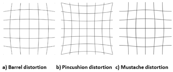
Radial distortion in entocentric (common) camera: a) Barrel distortion, b) Pincushion distortion, c) Mustache distortion

Fig. 2

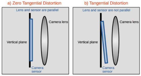
Tangential distortion is produced when the lens is not parallel to the image plane (the camera sensor)

Since the severity of the distortion is related to the principal point, thus, lessen its effect at the image center, often only the center region of the image is used generally for the measurement to ensure accuracy. This proves disadvantageous in the industrial environment. To address this problem, with regard to all non-uniform distortion patterns in the image, a method that is accurate, fast, robust, easy to calibrate for all types of camera and have a wide working area, has been proposed using the power of Deep learning, in particular, Deep Regression Neural Network.

2. Method

2.1 Classical Image Undistorting and Measuring Process

Commonly, the first step to undistort an image is to calibrate the camera. Typically, a calibration chessboard with measured patterns is used to find all the key features (the corners where the black tiles touch each other's). Then, from these key features in the pixel plane and the actual distances between features point in the real world, the intrinsic and extrinsic parameters of the camera and the relative location of the object compared to the camera can be calculated.^12-18 Then, using these parameters, the ratio of the measured dimension to its true dimension can be established with:

φ π = f x, I x, E x

(1)

where x = (x_pixel, x_realworld) is the coordinate of key features in the pixel plane and in the real world, I(x) is the intrinsic parameters and E(x) is the extrinsic parameters.

Then, the corrected estimate of the true dimension, $D ´$ , can be calculated by:

D ´ = D i φ π

(2)

where D_i is the initial dimension measured in the pixel plane.

2.2 Neural Network Measuring Process

Instead of using an approximation undistort model such as the Brown–Conrady model then some other function for warp perspective task in Eq. (1), a Neural Network can be used as a general mapping procedure between the input x and the output corrected estimate of the true dimension in Eqs. (1) and (2).

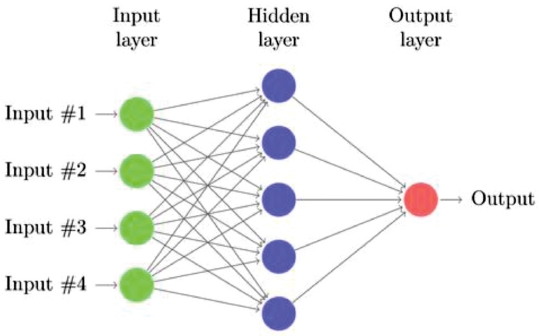
A neural network is represented in Fig. 3 where there are multiple nodes in a layer and multiple layers in a network.

Fig. 3

A simple neural network

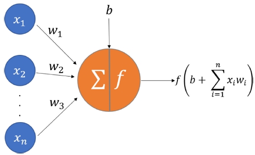
The first layer of the network has the same number of nodes as the number of input (For example: 2 points × 2 coordinate = 4 input features). For a simple Multi-Layer Perceptron (MLP) network, each output of the layer is the input of the next layer. In each node of the network, the input is processed through a linear function:

z i = ∑ j w i j a j + b i

(3)

where i is the index of the current node, j is the index of one of the nodes in the previous layer, w_ij is the weight to be optimized between node i and j, a_j is the output of node j and b_i is the bias value of this node.

Fig. 4

A Neuron passing the weighted sum of all the inputs through the non-linear Activation function

Next, the result of this linear equation is passed through a non-linear equation, for example, a Rectifier Linear Unit (ReLU):

a j = max ⁡ 0, z i

(4)

Then, the value a_j will be passed into the next layer and stop at the output node, where the value of the output node is the model's predicted value.

Since a Neural Network is a stack of multiple Non-linear functions on top of each other, it has the ability to search for a highly Non-linear solution, which can solve multiple complex problems very effectively. The method for a Neural Network to search for the desired solution that can map the input X to the output y, in this case, mapping the coordinate in the pixel plane to the actual distance between two point in the real world, is to define a loss function that represent the difference between the network's output y' and the target y. For a regression problem, the loss function chosen is often Mean Square Error, but in this experiment, the author chose Mean Absolute Error to compare the result with previous research:

L o s s = 1 n ∑ i = 0 1 y' i - y i

(5)

where n is the number of samples in the dataset, y'_t is the model prediction and y_i is the actual target of sample i.

To obtain a network that can represent the desired solution, one need to optimize all parameters w_ij and b_i in Eq. (3) so that the Loss value in Eq. (5) is the smallest possible. Then, this network is ‘trained’ with a randomly initialize the weight w_ij. Next, the Loss value between the model output and the actual output is calculated. This value will be used with the Back-Propagation method, using a Gradient Descent based strategy, to find the gradient of each w_ij and b_i in the network. In other words, the information on how to update each w_ij and b_i to lower the Loss value is now available for the optimizer, which would run the weights update procedure recursively until some terminated criterion is satisfied. The resulting network then would provide a function that replaces Eqs. (1) and (2).

The model used to generalize the distortion of the image and measured the distance between each pair is built with Keras and Tensorflow library. After the process of Hyper parameters tuning, the proposed Neural Network’s hyper-parameters is shown in Table 1 and the parameters for the OpenCV sub-pixel function in Table 2.

Table 1

The Structured light Scanner information

Table 2

Hyper-parameters for training model

2.3 Data Preparation

One of the main requirements to establish a working Deep Neural Network is that it need to have enough data. When the pattern is too complex for a small dataset to represent, the network would fail to generalize the pattern due to over-fit (the amount of noise in data is high) or under-fit (the amount of data is not enough to represent the pattern needed to learn).

A similar method for measuring geometric distance using Neural Network was proposed by Chao-Ton Su, et al.,¹⁹ but it did not have enough data for the network to formulate a generalized solution, thus, its solution is very target-dependent and camera-dependent.

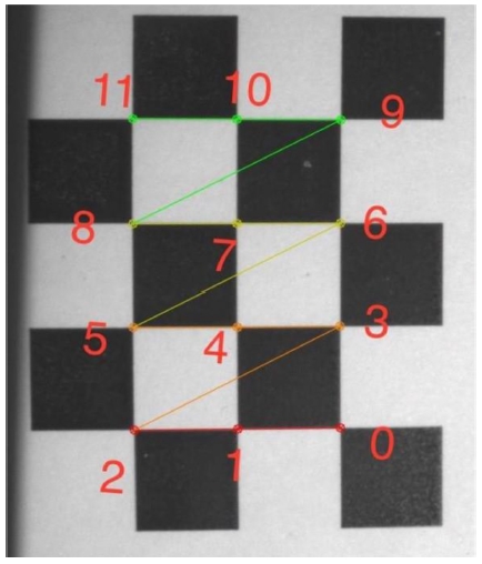
In order to provide a large dataset for the network (more than 10,000 input-output pairs in this case), the author used a printed chessboard pattern calibration board as the data generating source. First, the distances between the key features in the calibration board are measured. In this experiment, a 4 × 5 printed chessboard is used to detect M = 12 key features shown in Fig. 5. Then, the coordinate and the distance of each pair of key features would be used to train the Neural Network (For M = 12, there are C₂¹² = 66 pairs of key features in one image). Next, the chessboard images in N different locations is captured. For each image, M key features can be detected. Thus, the number of samples in the dataset is:

Fig. 5

An image of the calibration chessboard taken by the system with M = 12 detected key features

n = C 2 M × N

(6)

Note that, the N input images need to be varied in location so that all of the key features' coordinate in the pixel plane spread out most of the picture. The reason for this requirement is that there are different types of distortion in the image, each has a different effect on different areas of the picture. Without a high enough density of data point in the pixel plane, the dataset would not have enough information about the image distortion for the network to analyze and give a proper solution.

3. Result and Discussion

3.1 Result

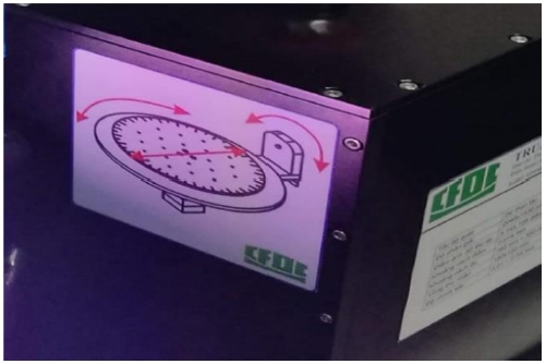
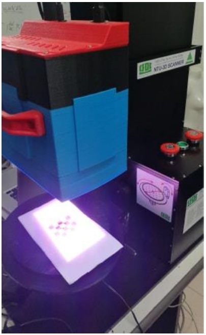
The equipment for the experiment is the Structure light Scanner using two High Dynamic Range cameras. These are the Point Grey Flea3 USB 3.0 cameras with M0814-MP2 lens (Fig. 7). More information about the Scanner can be found on Table 1 and Fig. 6.

Fig. 6

Scanner’s working table

Fig. 7

Scanner (CFOC) and chessboard in the experiment setup

Table 3

Parameters for sub-pixel function

About the printed chessboard, each tile has the side length approximating 10 mm. To increase the accuracy as well as to validate the measuring method, an assumption has been made that the actual distance between each pair of key features in Fig. 5 (For example: pairs (0,1), (0,2)) are values measured by the Universal microscopy UYM21 in the department of Precision Optical & Mechanical Engineering. For each of the 10-folds, the model is trained with 90% of the data (input: coordinate of a pair, output: distance measured by UYM21) and tested with the last 10% of the data.

3.1.1 Using 2 Images as Input

The experiment system consists of two cameras, located at the 20 degrees on the left and right of the z-axis. Thus, for each location of the calibrating chessboard, one would collected 2 input pictures, each contains C₂¹² = 66 pairs of input-output data (Fig. 5).

For this experiment, after removing invalidate input, the authors used 119 different positions, each with 2 photos captured from 2 camera. Using the 10-fold cross-validation testing procedure, the Mean Absolute Error (MAE) of the network is measured as 1.25 × 10^-2 mm with the standard deviation of 1.82 × 10^-3 mm.

3.1.2 Using 10 Images as Input

Instead of only capturing images in the 0-degree plane, another experiment is conducted with the angle between the plane holding the calibration board and captured the images at -10, -5, 0, 5 and 10 degrees.

Some hyper-parameters of the network are also changed such as the number of epochs is 300,000, the Optimizer is Adam²⁴ since empirical result shows that this setup would help the model converge faster and have higher accuracy.

For this experiment, after removing invalidate input, the dataset consists of 44 different positions, each taken with 5 different angles of the plane, with 2 photos captured from 2 camera. Using the 10-folds cross-validation testing procedure, the Mean Absolute Error (MAE) of the network is measured as 1.24 × 10^-2 mm with the standard deviation is 1.63 × 10^-3 mm.

Table 4

MAE results for 2 images input experiment

Table 5

MAE results for 10 images input experiment

3.2 Discussion

Besides from the experiment results shown in 3.1, the proposed measuring method is tested with the same input, but the output, the distance between each key features pair, is not measured but calculated with the assumption that all tiles edges are 10 mm in length and all vertical lines are perpendicular to all horizontal lines. The results are impressive, with Mean Absolute Error (MAE) of the network is 4.32 × 10^-5 mm with the standard deviation is 4.41 × 10^-5 mm. This suggesting that the proposed method is a new and viable way to measure in 2D dimensions.

In previous researches, Chao-Ton Su, et al.¹⁹ achieved the best accuracy with MAE in range of 1.00 × 10^-3 to 2.20 × 10^-3 mm. Qiucheng Sun⁷ also have a good result with MAE is 4.5 × 10^-3 mm. Bin Li⁸ measured the systematic error is less than 1.00 × 10^-3 mm and Yong Wang⁶ results in 2.00 × 10^-2 mm. While it seems that the previous researches yield better results than the proposed method of measurement (MAE is 1.24 × 10^-2), this method still has some advantages over the others:

(1) The experiment used a relatively low-quality camera compare to laboratory standard. Still, this method leveraging the ability of others measuring system (the Universal microscopy UYM21) to achieve better accuracy than the camera resolution (~0.1 mm per pixel).

(2) The proposed method is part independent and camera semi-independent. Which means, after the calibration process, this method can measure different parts without any further modification steps. It will also lower the importance of the camera quality in the system (since the accuracy also depends on the reference measuring system).

(3) The proposed method has uncertainty equal to zero (it would always yield the same result with the same input).

In the process of training and evaluating the model, the result showed that the higher the training time, the lower the Mean Absolute Error on both training dataset and validating dataset. Furthermore, the gap between training and validating loss throughout all 300,000 training epochs was always small, suggesting that the model had not converged yet. Thus, better training hardware than the GPU MSI GTX 1080 Titan 11 Gb with a proper hyper-parameter set and longer training time would most likely result in an even smaller error rate.

To improve the accuracy of this system without improving the camera and lens, a standardized and measured calibrated chessboard can be used. This will give more accurate labels to train and test the network.

Through the experimenting process, the authors notice that this Deep Regression system is very sensitive to any form of regularization method. Different methods have been tried such as Batch Normalization,²⁵ Dropout,²⁶ and L2 Regularization but all of them significantly worsen the output.

Due to the ability to map any set of input-output, some practitioners may be tempted to structure a network to better calibrate the camera. Theoretically, one can make such network with the input is the pixel plane and the real-world coordinate of key features, the output is the Intrinsic and Extrinsic parameters. Using a customized loss function that measures the difference between the predicted coordinate of the camera calibrated with the output parameters, one could probably achieve a comparable or slightly better result than the classical way to calculate Intrinsic and Extrinsic parameters. However, since the classical calibration procedure (using Brown - Conrady model) still only account for the Radial and Tangential distortion, the improvements of this method will be limited.

In summary, a Neural Network based method has been developed to be used for part-independent planar-dimensions measuring system. The result shows that the Deep Regression model used in the experiment can improve the accuracy of a low-quality optical measuring system. This was done by using Deep Learning to search in the vast non-linearly solution space for a function to represent the system camera’s intrinsic parameters, extrinsic parameters and the distortions in the images with a calibration chessboard measured by a high-accuracy measuring system. For future research, one can try to make use of the power of Convolution Neural Network and Transfer Learning in the process of undistorting an image with a Neural Network that has the undistorted image taken by the telecentric lens and the input is the same image added with random distortion. Another research direction would be developing a Deep Regression model for correcting the 3D measurement of the existing system.

Acknowledgments

This paper was presented at PRESM 2019

We would like to express our gratitude to Center for Optoelectronics, National Center for Technological Progress (NACETECH), Vietnam for their generosity in lending us the experiment equipment. We also want to thank the Department of Precision Mechanical and Optical Engineering, Hanoi University of Science and Technology, Vietnam for supporting the research. Lastly, we would like to show our appreciation to NAL Vietnam JSC for letting us use the GPU for training our Network.

REFERENCES

Su, X. and Zhang, Q., “Dynamic 3-D Shape Measurement Method: A Review,” Optics and Lasers in Engineering, Vol. 48, No. 2, pp. 191-204, 2010. [https://doi.org/10.1016/j.optlaseng.2009.03.012]
Phillips, C. L., Silver, D. A. T., Schranz, P. J., and Mandalia, V., “The Measurement of Patellar Height: A Review of the Methods of Imaging,” The Journal of Bone and Joint Surgery, Vol. 92, No. 8, pp. 1045-1053, 2010. [https://doi.org/10.1302/0301-620X.92B8.23794]
Pan, B., Qian, K., Xie, H., and Asundi, A., “Two-Dimensional Digital Image Correlation for In-Plane Displacement and Strain Measurement: A Review,” Measurement Science and Technology, Vol. 20, No. 6, Paper No. 062001, 2009. [https://doi.org/10.1088/0957-0233/20/6/062001]
Liguori, C., Paolillo, A., and Pietrosanto, A., “An On-Line Stereo-Vision System for Dimensional Measurements of Rubber Extrusions,” Measurement, Vol. 35, No. 3, pp. 221-231, 2004. [https://doi.org/10.1016/j.measurement.2003.11.004]
Angrisani, L., Daponte, P., Pietrosanto, A., and Liguori, C., “An Image-Based Measurement System for the Characterisation of Automotive Gaskets,” Measurement, Vol. 25, No. 3, pp. 169-181, 1999. [https://doi.org/10.1016/S0263-2241(98)00076-1]
Wang, Y., Zhang, X., and Chen, M., “Application of Machine Vision for Geometric Dimensions Measurement, in: Advanced Graphic Communications,” Packaging Technology and Materials, Ouyang Y., Xu M., Yang L., and Ouyang Y., (Eds.), pp. 639-644, Springer, 2016. [https://doi.org/10.1007/978-981-10-0072-0_79]
Sun, Q., Hou, Y., Tan, Q., and Li, G., “A Planar-Dimensions Machine Vision Measurement Method Based on Lens Distortion Correction,” The Scientific World Journal, Vol. 2013, Article ID: 963621, 2013. [https://doi.org/10.1155/2013/963621]
Li, B., “Research on Geometric Dimension Measurement System of Shaft Parts Based on Machine Vision,” EURASIP Journal on Image and Video Processing, Vol. 2018, No. 1, Paper No. 101, 2018. [https://doi.org/10.1186/s13640-018-0339-x]
Pan, B., Yu, L., Wu, D., and Tang, L., “Systematic Errors in Two-Dimensional Digital Image Correlation due to Lens Distortion,” Optics and Lasers in Engineering, Vol. 51, No. 2, pp. 140-147, 2013. [https://doi.org/10.1016/j.optlaseng.2012.08.012]
Tsai, R., “A Versatile Camera Calibration Technique for High-Accuracy 3D Machine Vision Metrology Using Off-the-Shelf TV Cameras and Lenses,” IEEE Journal on Robotics and Automation, Vol. 3, No. 4, pp. 323-344, 1987. [https://doi.org/10.1109/JRA.1987.1087109]
Heikkila, J., “Geometric Camera Calibration Using Circular Control Points,” IEEE Transactions on Pattern Analysis and Machine Intelligence, Vol. 22, No. 10, pp. 1066-1077, 2000. [https://doi.org/10.1109/34.879788]
Zhang, Z., “A Flexible New Technique for Camera Calibration,” IEEE Transactions on Pattern Analysis and Machine Intelligence, Vol. 22, pp. 1330-1334, 2000. [https://doi.org/10.1109/34.888718]
Ricolfe-Viala, C. and Sánchez-Salmerón, A.-J., “Correcting Non-Linear Lens Distortion in Cameras without Using a Model,” Optics & Laser Technology, Vol. 42, No. 4, pp. 628-639, 2010. [https://doi.org/10.1016/j.optlastec.2009.11.002]
Ricolfe-Viala, C. and Sánchez-Salmerón, A.-J., “Using the Camera Pin-Hole Model Restrictions to Calibrate the Lens Distortion Model,” Optics & Laser Technology, Vol. 43, No. 6, pp. 996-1005, 2011. [https://doi.org/10.1016/j.optlastec.2011.01.006]
Brown, D. C., “Decentering Distortion of Lenses,” Photogrammetric Engineering and Remote Sensing, Vol. 32, No. 3, pp. 444-462, 1966.
Fitzgibbon, A. W., “Simultaneous Linear Estimation of Multiple View Geometry and Lens Distortion,” Proc. of the 2001 IEEE Computer Society Conference on Computer Vision and Pattern Recognition, 2001.
Bukhari, F. and Dailey, M. N., “Automatic Radial Distortion Estimation from a Single Image,” Journal of Mathematical Imaging and Vision, Vol. 45, No. 1, pp. 31-45, 2013. [https://doi.org/10.1007/s10851-012-0342-2]
Jean-Yves Bouguet, “Camera Calibration Toolbox for Matlab,” http://www.vision.caltech.edu/bouguetj/calib_doc/, (Accessed 5 JUL 2019)
Su, C.-T., Chang, C. A., and Tien, F.-C., “Neural Networks for Precise Measurement in Computer Vision Systems,” Computers in Industry, Vol. 27, No. 3, pp. 225-236, 1995. [https://doi.org/10.1016/0166-3615(95)00024-8]
Clevert, D.-A., Unterthiner, T., and Hochreiter, S., “Fast and Accurate Deep Network Learning by Exponential Linear Units (Elus),” Proc. of ICLR, 2016.
Glorot, X. and Bengio, Y., “Understanding the Difficulty of Training Deep Feedforward Neural Networks,” Proc. of the 13th International Conference on Artificial Intelligence and Statistics, pp. 249-256, 2010.
Tieleman, T. and Hinton, G., “Lecture 6.5-rmsprop: Divide the Gradient by a Running Average of Its Recent Magnitude,” COURSERA: Neural Networks for Machine Learning, Vol. 4, No. 2, pp. 26-31, 2012.
Huang, G., Li, Y., Pleiss, G., Liu, Z., Hopcroft, J. E., et al., “Snapshot Ensembles: Train 1, Get M for Free,” Proc. of ICLR, 2017.
Kingma, D. P. and Ba, J., “Adam: A Method for Stochastic Optimization,” Proc. of 3rd International Conference for Learning Representations, 2015.
Ioffe, S. and Szegedy, C., “Batch Normalization: Accelerating Deep Network Training by Reducing Internal Covariate Shift,” https://arxiv.org/pdf/1502.03167.pdf, (Accessed 7 JUL 2019)
Srivastava, N., Hinton, G., Krizhevsky, A., Sutskever, I., and Salakhutdinov, R., “Dropout: A Simple Way to Prevent Neural Networks from Overfitting,” The Journal of Machine Learning Research, Vol. 15, No. 1, pp. 1929-1958, 2014.

Thang Duong Nhat

AI Team leader at NAL Vietnam JSC, Bachelor of Mechatronics Engineering, Hanoi University of Science & Technology. His research interest is Deep learning/ Machine learning.

E-mail: duongnhatthang@gmail.com

Binh Nguyen Duc

Undergraduate in the Department of Mechatronics Engineering, Hanoi University of Science & Technology. His research interest is using Machine Learning/Deep Learning techniques to apply for mechanical systems.

E-mail: binh.nd140377@sis.hust.edu.vn

Phuong Le Khac

Undergraduate in the Department of Mechatronics Engineering, Hanoi University of Science & Technology. His research interest is applying Machine Learning/Deep Learning techniques for mechanical systems.

E-mail: phuong.lk143509@sis.hust.edu.vn

Ngoc Tu Nguyen

Ph.D. Candidate - Department of Precision Mechanical and Optical Engineering, Hanoi University of Science & Technology. His research interest is 3D reconstruction.

E-mail: ngoctu@cfoc.vn

Mai Nguyen Thi Phuong

Assoc. Professor in the Department of Precision Mechanical and Optical Engineering, Hanoi University of Science & Technology. Her research interest is surface engineering and system design.

E-mail: mai.nguyenthiphuong@hust.edu.vn

No.	Characteristic	Value
1	Camera scanner system	2 cameras and 1 projector
2	Scanning time	2 s/time
3	System resolution	2048 × 1536
4	Maximum number of 3D pixels obtained	3.145.728 pixels
5	Average distance of points	0.014 mm
6	Working area	180 × 120 mm
7	Distance from working area to camera scanner system	250 ÷ 450 mm
8	Accuracy	0.013-0.03 mm
9	Scanning technique	Structured light (white light) is analyzed using “Three-step phase-shifting algorithm by Zhang, et al.
10	Working range	Yaw: 360 degrees. Pitch: 20 degrees. Z-axis: 100 mm

Name	Value
Calibration chessboard size	(3, 4)
Number of different positions	120
Number of nodes in each layer	(1024, 512, 256, 128, 64, 32)
Batch size	1024
Number of training epochs	5000
Dropout²⁶	0
L2 regularization	0
Loss	Mean absolute error
Activation function	Exponential linear unit²⁰
Kernel initializer	Glorot uniform²¹
Optimizer	RMSprop²²
Optimization strategy	Snapshot ensemble²³ (5 snapshots)
Test method	10-fold cross-validation

Name	Value
win-size	1
max-iteration	30
Epsilon	1 × 10^-9

Name	Value (mm)
Fold 1 MAE	1.14 × 10^-2
Fold 2 MAE	1.20 × 10^-2
Fold 3 MAE	1.20 × 10^-2
Fold 4 MAE	1.23 × 10^-2
Fold 5 MAE	1.76 × 10^-2
Fold 6 MAE	1.11 × 10^-2
Fold 7 MAE	1.23 × 10^-2
Fold 8 MAE	1.34 × 10^-2
Fold 9 MAE	1.12 × 10^-2
Fold 10 MAE	1.19 × 10^-2
Mean	1.25 × 10^-2
Population Standard Deviation	1.82 × 10^-3

Name	Value (mm)
Fold 1 MAE	1.28 × 10^-2
Fold 2 MAE	1.12 × 10^-2
Fold 3 MAE	0.92 × 10^-2
Fold 4 MAE	1.43 × 10^-2
Fold 5 MAE	1.37 × 10^-2
Fold 6 MAE	1.52 × 10^-2
Fold 7 MAE	1.26 × 10^-2
Fold 8 MAE	1.21 × 10^-2
Fold 9 MAE	1.13 × 10^-2
Fold 10 MAE	1.17 × 10^-2
Mean	1.24 × 10^-2
Population standard deviation	1.63 × 10^-3