Application of Bat algorithm for Improvement of Surface Integrity in Turning of AISI 304 Austenitic Stainless Steel
Copyright © The Korean Society for Precision Engineering
This is an Open-Access article distributed under the terms of the Creative Commons Attribution Non-Commercial License (http://creativecommons.org/licenses/by-nc/3.0) which permits unrestricted non-commercial use, distribution, and reproduction in any medium, provided the original work is properly cited.
Abstract
Improving product quality is a crucial factor in determining the competitiveness and business efficiency of enterprises. This study investigates the influence of the cutting parameters, including the cutting speed, the depth of cut, and the feed rate on the surface roughness and the residual stress during the turning of AISI 304 austenitic stainless steel. Moreover, the work aims to determine optimal cutting parameters to satisfy both surface roughness and residual stress requirements. The mathematical model of the relationship between the machining parameters and the performance characteristics was formulated based on the response surface methodology (RSM) and the Box–Behnken design of the experiments. Pareto optimal solution applying natural-inspired algorithm (Bat Algorithm) is proposed to solve the bi-objective optimization problem to obtain the lowest surface roughness and minimal residual stress. The optimum cutting parameters selected by the manufacturing planners from the Pareto optimal fronts are calculated to comply with the production requirements.
Keywords:
Bat algorithm, Response surface methodology, Surface integrity, Optimization, Pareto optimal1. Introduction
AISI 304 is the most common among grades of the austenitic stainless steel family, which accounts for roughly 72%. It has been widely used in high technology industries and chemical foods due to excellent corrosion resistance and high strength in high-temperature conditions.1 AISI 304 austenitic stainless steel is regarded as a difficult-to-machine material due to its low thermal conductivity, toughness, gumming, easy work hardening, and high built-up edge, leading to poor surface integrity, increased tool wear and low productivity.2 As a matter of fact, surface integrity is an essential criterion for evaluating a part's corrosion resistance and fatigue strength. More specifically, it is the surface roughness and residual stress which are two critical indicators of surface integrity determine the product's cost and quality.3 Improving surface integrity, therefore, is a requirement of the production and also a significant challenge for selecting technology parameters to satisfy customer requirements.4 Recently, researchers have been trying to develop new algorithms to optimize the machining process to ensure the above criteria simultaneously. Also, there has been a growing trend towards the application of nature-inspired algorithms to solve optimizations effectively. Yang proposed many nature-inspired algorithms, such as genetic algorithm (GA), particle swarm optimization (PSO), ant colony optimization (ACO), firefly algorithm (FA), cuckoo search (CS) and bat algorithm (BA).5
GA was applied to predict the surface roughness when milling and drilling. The test showed that the minimum surface roughness predicted by GA is lower than the results measured from the experiment, regression model and response surface method.6,7 Likewise, when turning AISI 304, tool wear estimated by the utilization of GA is lower than that calculated by applying traditional optimization techniques.8 Zhou, et al. also used the GA-GBRT technique to predict the surface roughness and optimize Ra and MRR simultaneously during the turning of AISI 304.9 The results indicated that increasing the machining efficiency requires a slight rise of the cutting speed and depth of cut. Kumar deployed a Pareto optimal solution based on the GA to identify optimum real-time condition, thereby simultaneously ensuring productivity and quality.10 When comparing the optimal results of surface roughness between GA and PSO, Ahmad, et al. emphasized that PSO brought about the lower optimal surface roughness in a shorter time than GA.11
On studying the algorithm used for soft computation in mechanical machining such as turning, milling, drilling and grinding, Chandrasekaran, et al. indicated that PSO with an unsophisticated mathematical structure was more efficient than GA in many circumstances.12 Besides, PSO combined with Pareto optimal solution was employed to find the minimum surface roughness and maximum plastic deformation layer thickness.13
When investigating optimization algorithms applied in many fields, BA is more novel, more simple and more robust than PSO.14,15 In multi-objective optimization, BA was also evaluated to be more effective than PSO, NSGA III.16
Based on the above literature review, it is noted that the metaheuristic algorithms have proved their superiority when solving the problem of multi-objective optimization in machining. BA has been proposed to be more effective in terms of a quick convergence rate, the optimal point's focus, and escape from local extremes. Therefore, this study focuses on two objectives. Firstly, RSM was used to develop the mathematical models of the relationship between cutting speed, feed rate, and depth of cut with two output indicators, including surface roughness and residual stress. Secondly, Pareto optimal solution based on applying BA was exploited to improve surface integrity when turning AISI 304 austenitic stainless steel. This paper’s findings were expected to help production planners choose the most suitable set of cutting parameters to meet customer requirements.
2. Experimental Procedure
2.1 Materials and Processes
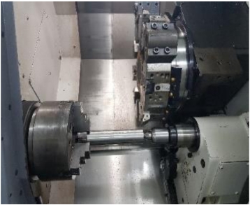
The experiment was conducted on Mori Seiki SL-253 CNC lathe, with a maximum spindle speed of 4,000 rev/min and a rated power of 28 kVA as shown in Fig. 1.
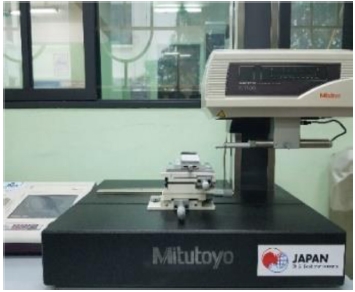
Mitutoyo Surftest SV-2100 surface roughness tester was used to determine surface roughness as shown in Fig. 2. The surface roughness of each experiment was the average value of the three measurements at three different points on the surface of each sample.
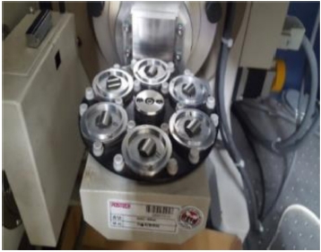
Residual stresses were determined through the X-Ray diffraction method (XRD) on a Rigaku D/Max 2,500/PC diffractometer as shown in Fig. 3. The X-Ray results were analyzed and calculated in combination with Williamson-Hall method to determine residual stress values.17
The experiments were carried out with the cutting tool Sanvik DCMT 11 T3 04-MF 2220 coated with CVD Ti (C, N) + Al2O3 + TiN.
AISI 304 austenitic stainless steel was chosen for the experiments. Tables 1 and 2 show the material's chemical composition and physical properties.
2.2 Design of Experiments
The experimental tests were carried out by employing Box-Behnken design (BBD) with three levels for each factor and the least total number of samples compared to central composite design (CCD) with 15 experiments.18,19 Based on the recommendations by the manufacturer of Sandvik Coromant and the results of the survey experiments, the ranges of cutting parameters and levels were selected as shown in Table 3 below.
RSM was then applied to develop a mathematical model of the relationship between independent inputs and output indicators.
Based on the number of operating variables investigated in this study, the experimental results obtained were fit for the second-order polynomial regression model19 using Eq. (1).
| (1) |
where y is the response function, ci, cii, cij are the coefficients of quadratic and linear constraint conditions, xi, xj are independent values.
3. Results and Discussion
The results of surface roughness and residual stress measurement are shown in Table 4. It can be seen that surface roughness and residual stress are in the range of (0.44-1.72) μm and (125.9-240.8) MPa respectively.
3.1 Analysis of Variance (ANOVA)
ANOVA determines the input parameters' significance level and their contribution to the outputs. ANOVA shows that a model is considered to be significant if the P-Value is less than 0.05, i.e., the significance of the model is at a 5% significance level as suggested by Kao and Green.20 In this study, Minitab software version 18 was used for the ANOVA. Tables 5 and 6 show the results of ANOVA fo Ra and σ respectively.
From the ANOVA tables, it is clearly stated that the feed rate is the parameter that most affects the surface roughness and residual stress with the contribution percentages of 86.22 and 41.64% respectively. Regarding P-Value, the cutting speed (0.566 for Surface Roughness and 0.522 for Residual Stress) and depth of cut (0.317 for Surface Roughness and 0.698 for Residual Stress) do not present any statistical significance on the two responses. This results are consistent with previous studies. Theoretically, the surface roughness is primarily a function of the feed rate and nose radius.21 Moreover, the higher the feed rate is, the greater the tensile residual stress on the surface is generated.22 Specifically, a rise in chip thickness leads to an increase in the temperature in the cutting zone, and the level of plastic deformation or hardening.
3.2 Develop Regression Equations
Based on Eqs. (1), (2) and (3) for prediction for surface roughness and residual stress were respectively formed as shown below.
| (2) |
| (3) |
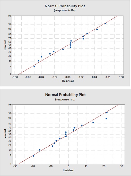
The Rsquare values (91.62 and 99.49%) for the quadratic and power models are high enough to obtain reliable estimates. Fig. 4 shows the normal probability plot of the residuals with values of surface roughness and residual stresses for normal distribution. Indeed, it can be seen that the points evenly distributed are skewed towards both sides in a straight line, which demonstrates the proposed model is sufficient to show the suitability.
3.3 Optimization of Responses
The objective of the present study is to minimize the surface roughness and residual stress simultaneously. The mathematical formulation of the current optimization problem can be stated as follows:
Minimize F(x) = {f1, f2}
where cutting parameters lower and upper bounds:
To optimize the multi-objective function, the article proposes to use the BA.
The bat algorithm (BA) is one of the nature-inspired algorithms proposed by Yang in 2010 based on the bats’ hunting behavior.23 In this algorithm, the bat’s position represents a solution. The algorithm’s goal is to find the best solution in all of the bat’s positions, including exploitation procedure and exploration procedure, such as:
- Exploitation procedure: The frequency fi, velocity vi and position xi of the ith bat at the iteration (t + 1) are defined by Eqs. (4), (5) and (6).
| (4) |
| (5) |
| (6) |
where, fmin, fmax are the minimum and maximum frequency of the bat populations, β ∈ [0,1] is a uniformly distributed random value and x* is the best location (Solution) after the tth iteration.
Exploration procedure: Random walks among bats are created around the best optimal to prevent getting block at a locally optimal solution by Eq. (7).
| (7) |
where, ε ∈ [-1,1] is a random number, At is the average loudness of all the bats at tth iteration.
The loudness and the rate of pulse emission have to be updated during the optimal search process, according to Eq. (8).
| (8) |
where, 0 < α < 1, τ are constants
This paper proposes a Pareto optimal concept, formulated by Vilfredo Pareto in the XIX century,24 using the BA to simultaneously optimize surface roughness and residual stress. The flow chart of the BA is shown in Fig. 5.
Parameters of the MOBA used in MATLAB are presented in Table 7.
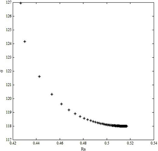
Fig. 6 shows the formation of Pareto optimal front that consists of the final set of solutions. The final optimum (Vc, f, ap) and their corresponding Ra and σ are shown in Table 8.
The Pareto optimal frontier points show that for each point corresponding to one set of parameters (Vc, f, ap), it is impossible to find another set of parameters (Vc, f, ap) for surface roughness to reach expected value that the residual stress is lower than the value on the Pareto front or vice versa, the residual surface stress is the desired value for which the surface roughness is lower than the present value. Indeed, in Table 8, if the parameter set includes Vc = 257.665 m/min, f = 0.090 mm/rev, ap = 0.229 mm, on the Pareto front, Ra = 0.461 μm, σ = 119.616MPa. This means that if Ra is expected to reach 0.461μm, it is impossible to choose any other sets of parameters (Vc, f, ap) so that σ is lower than 119.616 MPa.
Hence, based on specific requirements, the appropriate machining parameters are selected. For example, when required to achieve a lower surface roughness, the cutting parameters Vc = 262.242 m/min, f = 0.080 mm/rev, ap = 0.302 mm are chosen. The residual stress and surface roughness obtained then are σ = 126.941 MPa and Ra = 0.427 μm respectively. When a lower residual stress is required, the cutting parameters Vc = 252.779 m/min, f = 0.100 mm/rev, ap = 0.201 mm are selected. The residual stress and surface roughness are σ = 117.987MPa and Ra = 0.516 μm respectively.
This result is significant when compared to traditional optimization methods. RSM itself also finds the optimal set of parameters. Still, RSM gives only one result which is not as good as the result found by the BA. At the same time, Pareto optimal solution based on BA provides manufacturers with countless optimizations for different requirements.
3.4 Confirmation Test
With the predicted results found, it is necessary to conduct a confirmation experiment. One set of cutting parameters Vc = 257.665 m/min, f = 0.090 mm/rev, ap = 0.229 mm is selected for the verification experiment. According to the results shown in Table 9, it is possible to indicate that the prediction results are in good agreement with the experimental results with the error rate of only from 1.7 to 2.4%.
4. Conclusions
In this study, an experimental investigation was conducted to improve the surface integrity in terms of the surface roughness and residual stress when turning AISI 304 austenitic stainless steel. The following conclusions were drawn from the research.
ANOVA results showed that the feed rate had the most influence on surface roughness and residual stress.
Pareto optimal solution was employed based on the BA to optimize cutting parameters to minimize surface roughness and residual stress. Optimal results revealed the smallest roughness value is Ra = 0.427 μm; the minimum residual stress is σ = 117.987 MPa. The experimental confirmation results demonstrated that the Pareto optimal solution applying the BA was reliable and efficient.
Finding the optimal point on the Pareto front allows users to choose the optimal value for production requirements.
NOMENCLATURE
| MOBA : | Multi-Objective Bat Algorithm |
| ANOVA : | Analysis of Variance |
| AISI : | American Iron and Steel Institute |
| RSM : | Response Surface Methodology |
| Ra : | Surface Roughness |
| σ : | Residual Stress |
| Vc : | Cutting Speed [m/min] |
| f : | Feed Rate [mm/rev] |
| ap : | Depth of Cut [mm] |
| p : | Probability of Significance |
| F : | Variance Ratio |
| MS : | Mean of Squares |
| SS : | Sum of Squares |
| DF : | Degree of Freedom |
Acknowledgments
We would like to express our sincere thanks to the two anonymous reviewers for their valued comments. Also, we are very grateful to Department of Materials Science and Engineering, Pohang University of Science and Technology (POSTECH) and Vietnam-Japan Center, Hanoi University of Industry (HaUI) for supporting us to conduct such comprehensive experiments and accurate measurements.
REFERENCES
- Karunya, G., Ravikumar, P., Geeta Krishna, P., and Shiva Krishna, P., “Optimization of the Surface Roughness by Applying the Taguchi Technique for the Turning of AISI 304 Austenitic Stainless Steel,” International Journal of Mechanical Engineering and Technology, Vol. 8, No. 8, pp. 694-701, 2017.
- Sushil, I., Amit, P., and Rohit, P., “Machining Challenges in Stainless Steel-A Review,” International Journal of Advance Research, Ideas and Innovations in Technology, Vol. 3, No. 6, pp. 1395-1402, 2017.
-
Umbrello, D. and Filice, L., “Improving Surface Integrity in Orthogonal Machining of Hardened AISI 52100 Steel by Modeling White and Dark Layers Formation,” CIRP Annals, Vol. 58, No. 1, pp. 73-76, 2009.
[https://doi.org/10.1016/j.cirp.2009.03.106]

-
Zerti, O., Yallese, M., Zerti, A., Belhadi, S., and Girardin, F., “Simultaneous Improvement of Surface Quality and Productivity Using Grey Relational Analysis Based Taguchi Design for Turning Couple (AISI D3 Steel/Mixed Ceramic Tool (Al2O3 + TiC)),” International Journal of Industrial Engineering Computations, Vol. 9, No. 2, pp. 173-194, 2018.
[https://doi.org/10.5267/j.ijiec.2017.7.001]

-
Yang, X. S., “Nature-Inspired Optimization Algorithms,” Elsevier, 1st Ed., pp. 77-141, 2014.
[https://doi.org/10.1016/B978-0-12-416743-8.00010-5]

-
Kilickap, E., Huseyinoglu, M., and Yardimeden, A., “Optimization of Drilling Parameters on Surface Roughness in Drilling of AISI 1045 Using Response Surface Methodology and Genetic Algorithm,” The International Journal of Advanced Manufacturing Technology, Vol. 52, Nos. 1-4, pp. 79-88, 2011.
[https://doi.org/10.1007/s00170-010-2710-7]

-
Zain, A. M., Haron, H., and Sharif, S., “Application of GA to Optimize Cutting Conditions for Minimizing Surface Roughness in End Milling Machining Process,” Expert Systems with Applications, Vol. 37, No. 6, pp. 4650-4659, 2010.
[https://doi.org/10.1016/j.eswa.2009.12.043]

-
Amin, A., Haji Subir, S. A. B., and Arif, M. D., “Optimization of Tool Wear Using Coupled RSM-GA Approach in Turning of Stainless Steel AISI 304 with Magnetic Damping of Tool Shank,” Advanced Materials Research, pp. 117-121, 2015.
[https://doi.org/10.4028/www.scientific.net/AMR.1115.117]

-
Zhou, T., He, L., Wu, J., Du, F., and Zou, Z., “Prediction of Surface Roughness of 304 Stainless Steel and Multi-Objective Optimization of Cutting Parameters based on GA-GBRT,” Applied Sciences, Vol. 9, No. 18, Paper No. 3684, 2019.
[https://doi.org/10.3390/app9183684]

-
Kumar, S. L., “Measurement and Uncertainty Analysis of Surface Roughness and Material Removal Rate in Micro Turning Operation and Process Parameters Optimization,” Measurement, Vol. 140, pp. 538-547, 2019.
[https://doi.org/10.1016/j.measurement.2019.04.029]

-
Ahmad, N. and Janahiraman, T. V., “A Comparison on Optimization of Surface Roughness in Machining AISI 1045 Steel Using Taguchi Method, Genetic Algorithm and Particle Swarm Optimization,” Proc. of the IEEE Conference on Systems, Process and Control, pp. 129-133, 2015.
[https://doi.org/10.1109/SPC.2015.7473572]

-
Chandrasekaran, M., Muralidhar, M., Krishna, C. M., and Dixit, U., “Application of Soft Computing Techniques in Machining Performance Prediction and Optimization: A Literature Review,” The International Journal of Advanced Manufacturing Technology, Vol. 46, No. 5, pp. 445-464, 2010.
[https://doi.org/10.1007/s00170-009-2104-x]

-
Yue, C., Wang, L., Liu, J., and Hao, S., “Multi-Objective Optimization of Machined Surface Integrity for Hard Turning Process,” International Journal of Smart Home, Vol. 10, No. 6, pp. 71-76, 2016.
[https://doi.org/10.14257/ijsh.2016.10.6.08]

-
Talal, R., “Comparative Study between the (BA) Algorithm and (PSO) Algorithm to Train (RBF) Network at Data Classification,” International Journal of Computer Applications, Vol. 92, No. 5, pp. 16-22, 2014.
[https://doi.org/10.5120/16004-4998]

-
Khan, K. and Sahai, A., “A Comparison of BA, GA, PSO, BP and LM for Training Feed Forward Neural Networks in e-Learning Context,” International Journal of Intelligent Systems and Applications, Vol. 4, No. 7, pp. 23, 2012.
[https://doi.org/10.5815/ijisa.2012.07.03]

-
Perwaiz, U., Younas, I., and Anwar, A. A., “Many-Objective Bat Algorithm,” PLoS One, Vol. 15, No. 6, pp. 1-20, 2020.
[https://doi.org/10.1371/journal.pone.0234625]

-
Suryanarayana, C. and Norton, M. G., “X-Ray Diffraction: A Practical Approach,” Springer Science & Business Media, 1st Ed., pp. 63-237, 1998.
[https://doi.org/10.1007/978-1-4899-0148-4_3]

- Myers, R. H., Montgomery, D. C., and Anderson-Cook, C. M., “Response Surface Methodology: Process and Product Optimization Using Designed Experiments,” John Wiley & Sons, 4st Ed., pp. 369-542, 2016.
-
Bezerra, M. A., Santelli, R. E., Oliveira, E. P., Villar, L. S., and Escaleira, L. A., “Response Surface Methodology (RSM) as a Tool for Optimization in Analytical Chemistry,” Talanta, Vol. 76, No. 5, pp. 965-977, 2008.
[https://doi.org/10.1016/j.talanta.2008.05.019]

-
Kao, L. S. and Green, C. E., “Analysis of Variance: Is There a Difference in Means and What Does It Mean” Journal of Surgical Research, Vol. 144, No. 1, pp. 158-170, 2008.
[https://doi.org/10.1016/j.jss.2007.02.053]

-
Tebassi, H., Yallese, M., Khettabi, R., Belhadi, S., Meddour, I., et al., “Multi-Objective Optimization of Surface Roughness, Cutting Forces, Productivity and Power Consumption When Turning of Inconel 718,” International Journal of Industrial Engineering Computations, Vol. 7, No. 1, pp. 111-134, 2016.
[https://doi.org/10.5267/j.ijiec.2015.7.003]

-
Navas, V. G., Gonzalo, O., and Bengoetxea, I., “Effect of Cutting Parameters in the Surface Residual Stresses Generated by Turning in AISI 4340 Steel,” International Journal of Machine Tools and Manufacture, Vol. 61, pp. 48-57, 2012.
[https://doi.org/10.1016/j.ijmachtools.2012.05.008]

-
Yang, X. S. and He, X., “Bat Algorithm: Literature Review and Applications,” International Journal of Bio-Inspired Computation, Vol. 5, No. 3, pp. 141-149, 2013.
[https://doi.org/10.1504/IJBIC.2013.055093]

- Coello, C. A. C., Lamont, G. B., and Van Veldhuizen, D. A., “Evolutionary Algorithms for Solving Multi-Objective Problems,” Springer, 1st Ed., pp. 141-205, 2002.

Associate Professor in the Department of Mechanical Engineering, Hanoi University of Industry, Hanoi, Vietnam. ASC Bong’s research interest is advance materials and optimization processing machining.
E-mail: phamvanbong@haui.edu.vn

Ph.D. candidate in the Department of Mechanical Engineering, Hanoi University of Industry, Hanoi, Vietnam. He is interested in mechanical engineering, data analysis, simulation and optimization topics.
E-mail: hoitv@haui.edu.vn

