Realization and Scheduling of Free Spot Assembly Method for Machine Tools Using Cooperative Industrial Robots
Copyright © The Korean Society for Precision Engineering
This is an Open-Access article distributed under the terms of the Creative Commons Attribution Non-Commercial License (http://creativecommons.org/licenses/by-nc/3.0) which permits unrestricted non-commercial use, distribution, and reproduction in any medium, provided the original work is properly cited.
Abstract
The manufacturing industry is increasingly demanding flexible manufacturing and existing manufacturing methods with fixed equipment do not meet this requirement. The free spot assembly system is an ultra-flexible method that responds to this demand, enabling spatiotemporal free assembly by conveying all necessary resources with automated guided vehicles (AGVs). Although some studies have proposed free spot assembly, free spot assembly feasibility for assembling heavy objects, such as machine tools, by aligning them at high precision has not been verified. Work hour shifts, differences in worker skill levels, and cooperative work with robots have also not been considered in free spot assembly scheduling. This paper presents elemental technologies for realizing a free spot assembly system, with a scheduling method where a genetic algorithm is supported by dispatching rules with six genes. The computational results reveal the effectiveness of the proposed algorithm.
Keywords:
Assembly scheduling, Collaboration assembly, Cooperation assembly, Mobile robot, AGV1. Introduction
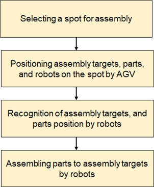
In the manufacturing industry, the demand for mass customization is increasing [1,2]. Reconfigurable manufacturing systems (RMS) have been studied for flexible production to meet this demand [3,4]. However, the flexibility of conventional fixed facilities is limited. As a new production system to solve this problem, free spot assembly systems, in which automated guided vehicles (AGVs) are used to set up assembly parts and equipment at an arbitrary location and then used as the base for assembly, have been considered. The entire process of the free spot assembly is shown in Fig. 1. Although some studies have proposed free spot assembly [5,6,7], free spot assembly feasibility for assembling heavy objects, such as machine tools, by aligning them at high precision has not been verified.
In free spot assembly, although the locations can be set arbitrarily, the scheduling becomes complicated, necessitating a scheduling system. There are examples of free spot assembly scheduling [8-10], but they do not consider worker work hour shifts, differences in worker skill levels, and cooperative work with robots. As assembly processes can be executed at different times of the day due to differences in worker shifts and skill levels, the work to set up and place the spots must be optimized dynamically. In addition, the optimal placement of robots with AGVs enables cooperative work among robots and between robots and workers, further increasing the flexibility of free spot assembly.
In this paper, we show elemental technologies for realizing a free spot assembly method in which cooperative industrial robots are introduced for assembling machine tools by verifying an actual machine. In addition, for optimal scheduling of free spot assembly, we propose a genetic algorithm with gene expression suitable for solving the features of this problem and confirm its usefulness by numerical experiments.
2. Examination of Elemental Technologies required for Free Spot Assembly of Machine Tools
In this section, elemental technologies required for free spot assembly of machine tools is shown. The first stage of fig. 1 is decided by the scheduling mentioned below in Chapter 3, and the spot setting is shown in Section 2.1. The required technologies in the second stage of fig. 1 is shown in section 2.2, the third in section 2.3, and the fourth in section 2.4, section 2.5.
2.1 Spot Setting
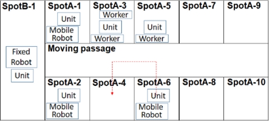
Figure 2 shows an overview of the free spot assembly of the machine tools under study. As shown in the figure, spots A-1 to A-10 and spot B-1 were set as spots. Spots A-1 to A-10 were spaces where a mobile robot and a worker could work cooperatively. Spot B-1 was the space where the fixed robot was installed, and mobile robots and workers could not work.
The main assembly targets of the machine tools were the bed and column, which were placed on AGVs and delivered to the desired spots. At the same time, the parts to be assembled on the bed and column were simultaneously delivered by AGVs to the required spots. Although, ideally, the space (position, size) of a spot could be freely and arbitrarily set, the position and size of a spot were treated as fixed in this study.
2.2 Position Recognition during Movement Control of AGVs
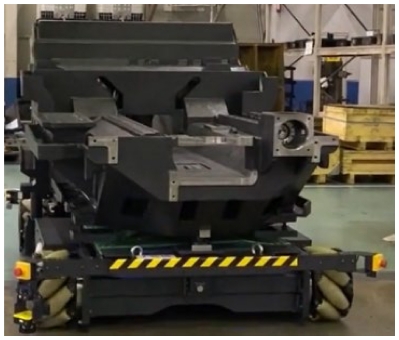
Figure 3 shows an AGV with a bed mounted. The tires of the AGVs were mecanum wheels, which enabled flexible movement in all directions. When moving an AGV, the position of the AGV must be recognized. In this study, two light detection and ranging (Lidar) devices were mounted on a single AGV, and the position of the AGV was recognized by the simultaneous localization and mapping (SLAM) method. In this case, the position recognition accuracy of the AGVs was ±10 mm, sufficient for moving and controlling the AGVs without interfering with other objects.
2.3 Position Recognition during Assembly
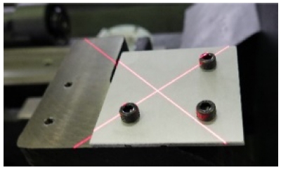
The position recognition accuracy of the AGVs was ±10 mm, which was not accurate enough to realize the assembly of parts. Therefore, a relative distance measurement camera was installed in the end-effector section of the robot mounted on the AGV. Furthermore, as shown in Fig. 4, a cross-shaped slit light was projected onto the position to be assembled after AGV movement to measure the position and inclination of the plane. The position recognition accuracy was ±0.1 mm, which was not sufficient for assembly. However, assembly with a position recognition accuracy of ±0.1 mm was made possible by the innovations described in Section 2.4.
2.4 Assembly Part Shape and Gripping Tool Shape
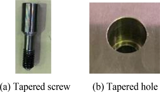
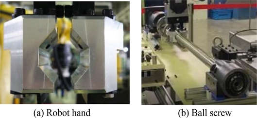
The position recognition accuracy by the camera was ±0.1 mm, while the error associated with the arm when the robot grasped the heavy object and the actual position recognition accuracy of the end-effector part of the robot was about ±0.5 mm. To realize assembly even with this accuracy, we devised a method to perform positioning according to the shape of the part to be assembled. As an example, Fig. 5 shows a screw of an assembled part. As shown in the figure, tapers are provided at the tip and center of the screw so that the axes of the bolt screw and nut screw are aligned. In addition, as shown in Fig. 6(a), when gripping a ball screw, the shape of the gripper attached to the end-effector was made hexagonal when gripped so that even if the position recognition accuracy of the end-effector part was ±0.5 mm, the ball screw could be gripped stably as shown in Fig. 6(b) of the same figure. After the ball screw was installed by the robot, the final position adjustment was performed by the worker.
2.5 Cooperative Work at the Same Spot
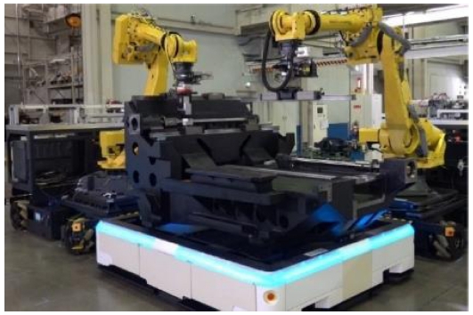
By moving the robot installed on the AVG and the worker to the same spot, the robot and worker, or multiple robots, simultaneously worked on the same part at the same spot. This is called cooperative work. Using an actual machine, we verified that cooperative work was possible in the assembly of machine tools. Figure 7 shows two robots performing cooperative work assembling a bed. As the size of the bed varied depending on the model, the placement of the two robots on the bed also differed. However, we confirmed that the robots were placed at the optimal position by the AGVs and that cooperative work was conducted without interference.
3. Scheduling Method
To effectively operate the free spot assembly method, it was necessary to efficiently schedule the assembly. In the following sub-section, we describe our proposed scheduling method.
3.1 Scheduling Model
The detailed conditions of the scheduling model in this study were set as follows:
- • There were 10 spots that could be worked by a worker and a mobile robot
- • The worker’s day shift was 4 hours of continuous work starting at 8:00 a.m., followed by a break, then 4 hours of continuous work starting at 12:45 p.m.
- • The night shift was 4 hours of continuous work starting at 4:45 p.m., followed by a break and 3.5 hours of continuous work starting at 9:30 p.m.
- • There were three workers on the day shift and three on the night shift
- • The number of AGVs capable of carrying bed columns was 16
- • There was one mobile cooperative industrial robot
- • There were two mobile non-cooperative industrial robots (Robots that cannot cooperate with operators)
- • Bed and column assembly was performed by two fixed robots at a spot (the two fixed robots performed the operation synchronously, so they were treated as one fixed robot for scheduling purposes).
The following scheduling model was applied to the detailed scheduling conditions above:
The bed and column were assembled separately and then joined together. A job was defined as the assembly of one machine tool, and a job consisted of several operations, where each operation was performed by one worker or one robot.
An operation was performed at any one spot. The worker and the mobile robot performed the operation at any spot A in Fig. 2. The operation of joining the bed and the column was performed by the stationary robot at spot B.
Assembly operations for different beds and different columns could be performed simultaneously. In addition, in any given spot, in the assembly operation for one bed or one column, some operations could be performed by two workers, one worker and one mobile cooperative industrial robot, and two robots in cooperation. Non-cooperative industrial robots were not allowed to cooperate with workers due to functional limitations.
The practicable skill levels of the workers were defined, and the execution time of an operation varied depending on the skill. Furthermore, workers were assigned shifts and not allowed to execute operations outside their shifts. The robots could work 24 hours a day. Each robot had a payload function that determined which operations it could and could not perform.
When a robot moved to another spot after executing an operation, a travel time was calculated. For example, when a robot moved from SpotA-6 to SpotA-4 as shown by the red line in Fig. 2, the travel time was calculated as if the robot had moved at the specified movement speed from the center of SpotA-6 to the center of SpotA-4 via the center of the aisle. A travel time was likewise calculated for the operator. The bed or column was transported between the spots with the bed or column mounted on an AGV, while assembly operations were executed with the bed or column mounted on an AGV. The travel time was also calculated if a bed or column operation was completed at one spot and another operation was executed at another spot. Collisions along the way during AGV travel were not considered.
The AGVs carrying the column when the bed and column were joined, or the AGVs when assembly was completed and the assembled goods placed in storage, were released from the assembly operations. The number of AGVs transporting beds and columns was limited. If a bed or column being assembled needed to wait for an operation, it was placed in a spot where no work was taking place (standby). In standby, multiple AGVs were allowed to be placed in one spot. There were 16 AGVs, 3 mobile robots (1 mobile cooperative industrial robot and 2 mobile non-cooperative industrial robots), 3 workers each for the day and night shifts, and 10 spots, and we considered that the number of spots was sufficient for the elements to be placed in the spots. The scheduling of placement spots for the beds and columns awaiting processing did not need to be considered.
3.2 Scheduling Policy
When the bed and the column were joined, the shorter the time difference between the completion of each assembly operation, the shorter the time was that the bed waited for the column or that the column waited for the bed, and thus the more efficient the spot utilization and AGV utilization became. In this study, where the work of the workers and the robots were intermingled, it was important to use the AGVs efficiently to keep the robots running during the night when the operators were not available. In addition, considering the assembly efficiency at all spots, the mobile robots moved to other spots as necessary during the assembly operation at each spot and performed the assembly operations.
3.3 Scheduling Genes
In this study, we developed a scheduling system using a genetic algorithm with multiple classes of genes to efficiently search for the optimal schedule for the scheduling model described above. A description of the multiple classes of genes that realize the aforementioned scheduling policy is given below.
Jobs were represented by genes that were assigned to six classes. The six classes were composed of “(1) processing sequence for each job,” “(2) processing sequence for each operation,” “(3) cooperative process for each operation,” “(4) assigned worker number for each operation,” “(5) assigned robot number for each operation,” and “(6) assigned spot number for each operation”, which were real numbers or integers depending on the class [11,12]. Genes of each class were assigned as follows:
① Processing sequence for each job
Following the scheduling policy described above, we wanted to shorten the difference between the times when the bed and column assembly processes were completed. However, if the processing times of the bed and the column were identical, the free spot assembly flexibility might have been lost unless it was possible to switch the processing sequence with an operation belonging to another job when the processing sequences of the bed and column processes were too close. Therefore, to maintain the flexibility of the processing sequence of the processes and to suppress the increase in scheduling time, we limited the range in which the processing sequence of the processes belonging to different jobs could be swapped. The details are described in “(2) Processing sequence for each operation”.
② Processing sequence for each operation
When scheduling, the processing sequence of an operation could be represented by a processing sequence gene assigned to the process. However, in this study, to limit the range of interchangeability of the processing sequences of processes belonging to different jobs, we assigned processing sequence genes to the jobs and combined these with processing sequence genes assigned to the operations, which were thereby expressed as the processing sequences of the operations. Table 1 shows examples of the processing sequences of operations and the six classes of genes in three job examples. It can be seen that the processing sequence of an operation was the sum of the values of the “(1) Processing sequence for each job” gene and the “(2) Processing sequence for each operation” gene, thus becoming more prone to triggering swapping of process orders for processes belonging to different jobs; thus, the larger the range of possible values of the processing sequence gene assigned to an operation, the larger the likelihood of switching the processing sequence of operations belonging to different jobs. By setting the range of values of the processing sequence gene assigned to an operation and the gene assigned to a job in advance, it was possible to determine the likelihood of switching the processing sequence of operations belonging to different jobs. Here, using the processing sequence adjustment values a, b, and g, the processing sequence genes assigned to the operation were in a range from -a to a, and the processing sequence genes assigned to the job were from b to g -b. The processing sequences thereby had a range of b - a to g - b + a. In this study, assuming g = 1 and b = a, the processing sequence of the operation was set to be in the range 0 to 1, and a was assumed to have a range of 0 to 0.5.
If a was close to zero, the processing sequences belonging to different jobs were not swapped, and only the processing sequences belonging to the same job were swapped. In contrast, if a was 0.5, the processing sequence genes assigned to jobs did not function, with only the processing sequence genes assigned to operations used. By setting a a suitable value that falls between 0 and 0.5, it was thought that a solution could be efficiently found.
The genes for “(2) Processing sequence for each operation” were arranged in the order of the bed operation, the column operation, and the operation after the bed and column were integrated. (The same applied to the genes of each class described below.)
③ Cooperative process for each operation
Operations where cooperative work by operators and robots was possible were flagged. A gene of 1 for an operation indicated that the operation was cooperative, and a gene of 0 indicated that the operation was not cooperative. The operations were scheduled as cooperative only when both the genes of two cooperative processes were 1.
④ Assigned worker number for each operation
This is a gene that was assigned to an operation to be performed by a worker. When assigning an operation, it indicated the number of the worker to be assigned. The number of the worker is determined by the rank of skill value among the workers available for work in the time period.
⑤ Assigned robot number for each operation
This is a gene that was assigned to an operation to be performed by a robot. It indicated the number of the robot to be assigned.
⑥ Assigned spot number for each operation
This gene was assigned to an operation with multiple candidate spots to assign the process. It shows which number spot was assigned.
3.4 Gene Manipulation Process
The steps followed to manipulate the genes of the GA in this study are given below.
• Step 1: Create Np chromosomes at random, where Np is the number of individuals in each generation; this step is treated as the initial generation.
• Step 2: Transfer the best individuals to the next generation. The chromosomes for transfer to the next generation are then selected until the number of individuals in the next generation reaches Np/2. The tournament method is used to select the best chromosome among two randomly selected chromosomes. The next generation is then designated as the current generation.
• Step 3: Select two chromosomes from the current generation and mate them as parent chromosomes to generate two offspring chromosomes. This procedure is repeated until Np × 0.4 individuals are generated in Step 3. Uniform mating is applied as the mating method. For each gene of each of the six classes of chromosomes, the gene value is inherited from each of the two parental chromosomes with a probability of 50%.
• Step 4: Randomly select one of the chromosomes from the current generation and mutate it. This procedure is repeated until Np × 0.1 individuals are generated in Step 4. For each of the six classes of chromosomes, the mutation method randomly changes the value of the gene to the range of possible values for the chromosome with a probability of 5%.
• Step 5: If the number of generations reaches a preset value, the program terminates; otherwise, it returns to Step 2.
The time from scheduling to the end of all jobs, i.e., the “makespan” was used to evaluate the adaptability of each gene.
3.5 Dispatching Policy
The processes were dispatched based on the following rules 1 to 5.
• Rule 1: For each process, the processing sequence is determined and allocated based on the sum of the values of the genes “(1) Processing sequence for each job” and “(2) Processing sequence for each operation”. The worker, robot, and site to be allocated were determined by the values of the gene classes of “(3) Cooperative process for each operation,” “(4) Assigned worker number for each operation,” “(5) Assigned robot number for each operation,” and “(6) Assigned spot number for each operation”.
• Rule 2: If two operations can be processed at the same site without a time interval, the operations are processed at the same site regardless of the gene value of “(6) Assigned spot number for each operation”.
• Rule 3: Each operation is allocated to the earliest possible time.
• Rule 4: The first time a bed/column operation in a job is assigned, decide which AGV to assign to the bed/column operation. One AGV is released when the bed/column is integrated and the job is finished, with no processes from either the bed or column or from other jobs assigned to that AGV until the AGV is released.
• Rule 5: When assigning an operation to a job to which no operation has been assigned, assign the operation only when two or more AGVs are available. Simultaneously, reserve an AGV for either the bed or the column and do not assign another job to that AGV until then.
In the scheduling target of this study, two beds/columns before integration were assembled by sharing the same type of AGVs. Furthermore, the AGVs were not released until the steps were completed in one process. Due to its nature, if only one of the beds/columns of each job is allocated to an AGV and all the AGVs are occupied, the AGV cannot be released owing to the integration of the bed/column, resulting in a non-executable solution. Rule 5 prevents the creation of infeasible solutions.
4. Evaluation Experiments
Numerical experiments were conducted to confirm the effectiveness of the proposed scheduling method.
4.1 Experimental Conditions
In the experiment, we performed scheduling using the assembly of five machine tools as a case study. Figure 8 shows the assembly process of machine tools A, B, and C used as the case studies; the operations performed by the robot and the operator in the assembly of the bed and column are separately represented. A box indicated with a black frame in the figure represents one operation. The operations were processed in order from left to right. The arrows indicate a change in the work site. The orange boxes indicate worker operations. The yellow boxes indicate operations for non-cooperative industrial robots. The green boxes indicate operations that can be performed by either cooperative or non-cooperative industrial robots. The blue boxes indicate the processes for fixed robots. The two process groups surrounded by dotted lines arranged vertically indicate that the operations in the upper process group can cooperate with the operations in the lower process group. However, cooperative work was not possible with processes assigned to non-cooperative industrial robots and operations for workers. Machine tool D and machine tool E had the same assembly process as machine tool A, but the overall process times were 0.8 times and 1.4 times longer, respectively.
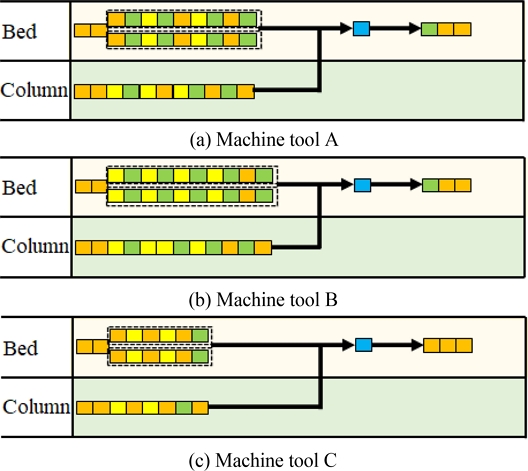
The assembly processes of machine tools are shown. The orange boxes indicate worker operations, yellow indicate non-cooperative industrial robots’ operations, green indicate robot’s operations, and blue indicate the fixed robots’ operations. The two process groups surrounded by dotted lines indicate cooperative work.
The worker’s working time was defined as the standard working time of the operation divided by the worker’s skill value. The skill values of the workers were 1.3, 1.0, and 0.6 for the three day-shift workers and 1.2, 0.9, and 0.7 for the night-shift workers, respectively.
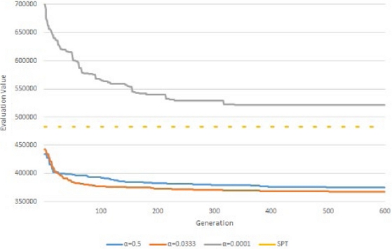
The genetic algorithm proposed in this study was used for scheduling with three different values for the processing sequence adjustment value a : 0.0001, 0.0333, and 0.5. For the case where a = 0.0001 and therefore close to 0, swapping of processing sequences between different jobs was almost eliminated. In contrast, when a was 0.5, the class of “(1) Processing sequence for each job” did not function at all. The above two patterns can be expressed practically without bringing up a; a = 0.0333 was set as the reciprocal of the number of jobs, assuming the number of jobs was 30, as it was an appropriate intermediate value.
The scheduling result is evaluated by makespan, and the time unit is one second. For comparison, we also performed scheduling using the shortest processing time (SPT) rule, in which dispatching was performed in the order of shortest process times without using the genetic algorithm.
4.2 Scheduling Results
Figure 9 shows the transition of the evaluation values for each number of generations of the genetic algorithm with a solid line when the number of jobs was 30, and the number of machine tools A to E assembled was 7, 6, 6, 6, and 5, respectively. For comparison, the evaluation values of SPT are also shown with dotted lines. Five test runs were conducted, and the average values are shown. The number of individuals in each generation of the genetic algorithm was Np = 3000, and the number of generations of the genetic algorithm was 600, according to the preliminary experiments. The computation time of the genetic algorithm was 50 hours per trial on a PC with an Intel Xeon E-2640 CPU v3@2.60 GHz and 32 GB memory.
The pattern achieved with a = 0.0001 had the worst evaluation value, confirming that a should not be too small. The patterns achieved with a = 0.0333 and a = 0.5 yielded better results than SPT for the initial generation. The pattern for a = 0.0333 was equivalent to that for the a = 0.5 up to 20 generations but was significantly better than that achieved with a = 0.5 at 100 generations. Furthermore, it yielded better results than those achieved with a = 0.5 at 600 generations when the search was advanced.
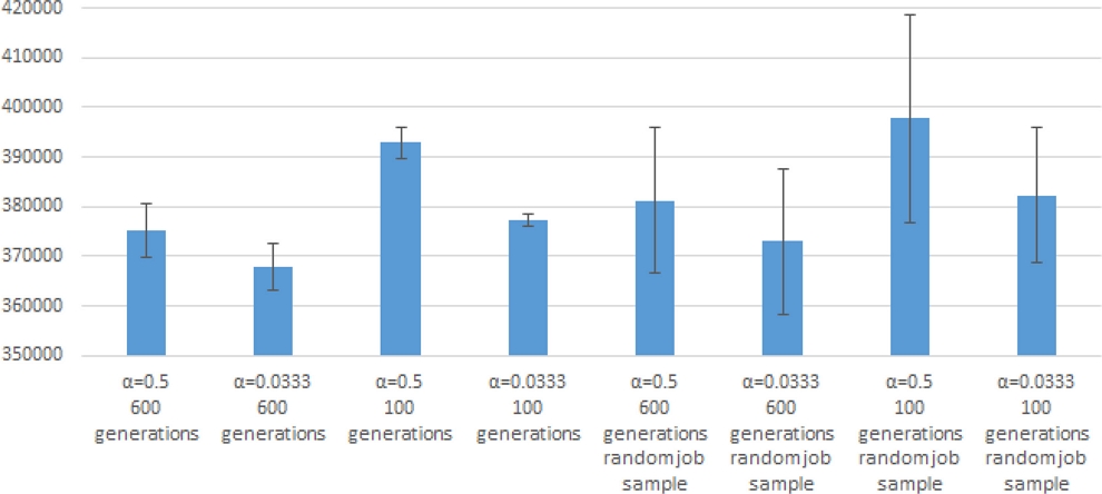
The left four bars in fig. 10 shows the means and standard deviations of the patterns for a = 0.0333 and a = 0.5 at 100 and 600 generations, respectively. a = 0.0333 was still better on average at 600 generations, but a = 0.0333 was much better at 100 generations, including its standard deviation.
As examples of the different combinations of jobs, we created five job combinations in which the number of jobs was 30 and the assignment of machine tools A to E to each job was randomly determined; we performed scheduling for these job combinations. The right four bars in fig. 10 show the mean values and standard deviations of the patterns achieved with a = 0.0333 and a = 0.5 for 100 and 600 generations, respectively. The standard deviations were naturally larger because the job combinations were different, but we could confirm that a = 0.0333 was better on average, especially at 100 generations.
From these results, there is room for research on the optimal a value, but we confirmed that using a is better because a = 0.0333 is better than a = 0.5, which can be expressed without a by just disusing the class of “(1) Processing sequence for each job”. The reciprocal of the number of jobs will be better try of a value. It is assumed that using a is effective because it shortens the time difference between the completion of bed and column operation, and contribute to using a limited number of AGVs efficiently to keep the robots running during the night when the operators were not available.
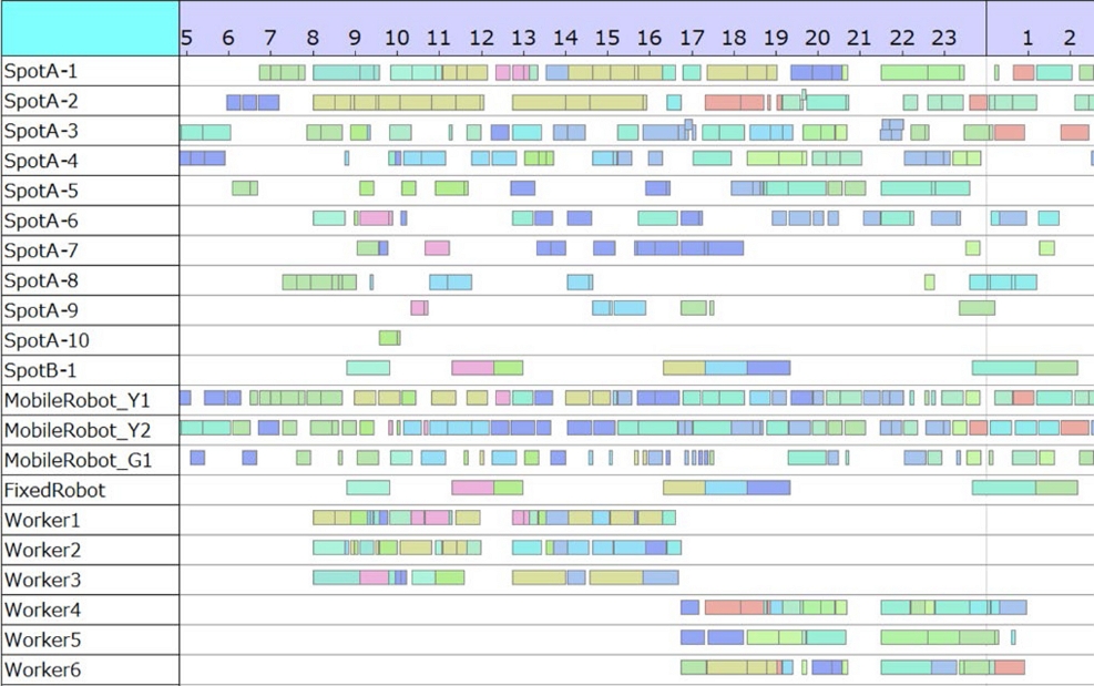
Figure 11 shows a Gantt chart of some of the scheduling results obtained. The horizontal axis represents time, while the bars in the Gantt chart represent the state in which a bed or a column is placed at each spot and the state in which a robot or a worker is working. The color of the bar indicates the differences between the jobs.
5. Conclusions
In this paper, we proposed free spot assembly in which multiple workers and robots work cooperatively and collaboratively. The elemental technologies for realizing free spot assembly in machine tools were verified on actual machines, and the feasibility of the free spot assembly was demonstrated.
Furthermore, we proposed a scheduling method for efficient free spot assembly and confirmed its effectiveness through numerical calculations. In the proposed method, the machine tool assembly process was represented by the following genes: “(1) Processing sequence for each job,” “(2) processing sequence for each operation,” “(3) cooperative process for each operation,” “(4) assigned worker number for each operation,” “(5) assigned robot number for each operation,” and “(6) assigned spot number for each operation. The process processing sequence adjustment value a was used as a parameter. We realized a schedule based on the adaptability evaluation value of the schedule.
We constructed a scheduling system based on the proposed method and conducted evaluation experiments. By setting the processing sequence adjustment value a to an appropriate value, we obtained a better evaluation, especially when the search time was relatively short.
REFERENCES
-
Tien, J. M., (2011), Manufacturing and services: From mass production to mass customization, Journal of Systems Science and Systems Engineering, 20, 129-154.
[https://doi.org/10.1007/s11518-011-5166-x]

-
Kokuryo, D., Kaihara, T., Kuik, S. S., Suginouchi, S., Hirai, K., (2017), Value co-creative manufacturing with IoT-based smart factory for mass customization, International Journal of Automation Technology, 11(3), 509-518.
[https://doi.org/10.20965/ijat.2017.p0509]

-
Koren, Y., Shpitalni, M., (2010), Design of reconfigurable manufacturing systems, Journal of Manufacturing Systems, 29(4), 130-141.
[https://doi.org/10.1016/j.jmsy.2011.01.001]

-
Li, X., Bayrak, A. E., Epureanu, B. I., Koren, Y., (2018), Real-time teaming of multiple reconfigurable manufacturing systems, CIRP Annals, 67(1), 437-440.
[https://doi.org/10.1016/j.cirp.2018.04.051]

-
Huettemann, G., Buckhorst, A. F., Schmitt, R. H., (2019), Modelling and assessing line-less mobile assembly systems, Procedia CIRP, 81, 724-729.
[https://doi.org/10.1016/j.procir.2019.03.184]

-
Michalos, G., Sipsas, P., Makris, S., Chryssolouris, G., (2016), Decision making logic for flexible assembly lines reconfiguration, Robotics and Computer-Integrated Manufacturing, 37, 233-250.
[https://doi.org/10.1016/j.rcim.2015.04.006]

-
Michalos, G., Kousi, N., Makris, S., Chryssolouris, G., (2016), Performance assessment of production systems with mobile robots, Procedia CIRP, 41, 195-200.
[https://doi.org/10.1016/j.procir.2015.12.097]

-
Buckhorst, A. F., Huettemann, G., Grahn, L., Schmitt, R. H., (2019), Assignment, sequencing and location planning in line-less mobile assembly systems, Tagungsband des 4. Kongresses Montage Handhabung Industrieroboter, 227-238.
[https://doi.org/10.1007/978-3-662-59317-2_23]

-
Buckhorst, A. F., Schmitt, R. H., (2020), Multi-staged, multi-objective optimization for operation management in line-less mobile assembly systems (LMAS), Procedia CIRP, 93, 1121-1126.
[https://doi.org/10.1016/j.procir.2020.04.046]

-
Buckhorst, A., do Canto, M., Schmitt, R., (2022), The line-less mobile assembly system simultaneous scheduling and location problem, Procedia CIRP, 106, 203-208.
[https://doi.org/10.1016/j.procir.2022.02.179]

-
Bean, J. C., (1994), Genetic algorithms and random keys for sequencing and optimization, ORSA Journal on Computing, 6(2), 154-160.
[https://doi.org/10.1287/ijoc.6.2.154]

-
Kaweegitbundit, P., Eguchi, T., (2016), Flexible job shop scheduling using genetic algorithm and heuristic rules, Journal of Advanced Mechanical Design, Systems, and Manufacturing, 10(1), JAMDSM0010.
[https://doi.org/10.1299/jamdsm.2016jamdsm0010]


Ph.D. candidate, Department of System Design Engineering, Keio University.
E-mail: inoueko@makino.co.jp

Professor, Department of System Design Engineering, Keio University.
E-mail: haoyama@sd.keio.ac.jp

