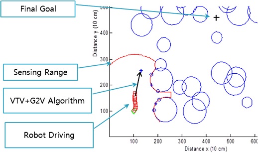
Minimizing Driving Risk of Mobile Robots by Combining a Goal Guidance Vector Algorithm with Reactive Navigation
Copyright © The Korean Society for Precision Engineering
This is an Open-Access article distributed under the terms of the Creative Commons Attribution Non-Commercial License (http://creativecommons.org/licenses/by-nc/3.0) which permits unrestricted non-commercial use, distribution, and reproduction in any medium, provided the original work is properly cited.
Abstract
In the navigation of mobile robots, the driving risk can be minimized by increasing the probability of success. The algorithm, which is currently commonly known as the shortest path algorithm, performs efficiently, but does not exhibit a good probability of success for achieving the final goal. In this paper, we develop a new reactive navigation algorithm, known as the goal guidance vector (G2V), which can minimize the driving risk within the sensing range. The G2V is designed to improve the performance of the reactive navigation algorithm using a hazard cost function (HCF) that accounts for the scale and locations of the obstacles within the sensing range. We also adopt real-time fuzzy reactive control to determine the weighting factors of the HCF in an unknown environment to determine the optimal G2V. Simulations are conducted to validate the use of this approach for various environments.
Keywords:
Reactive navigation, Goal guidance vector, Hazard cost function, Mobile robot, Minimize risk1. Introduction
The success probability of arriving at a final goal is a crucial factor in the autonomous navigation of a mobile robot. However, this technology for autonomous navigation falls short of our expectations because of the limitations of the on-board sensors (i.e., The Vision Sensor, The IR Sensor, Ladar, etc.) for environmental perception and imperfect algorithms. It is especially difficult to achieve the final goal using reactive navigation because of random motion and the environmental information obtained from the contact sensors.
The robot’s chosen optimal direction in reactive navigation is still difficult to execute within a structured map. Previous studies have produced what is now commonly known as the shortest path algorithm, in which the next location a robot moves to is determined using a sensing range such that the robot will move the shortest distance to the final goal. The shortest path algorithm performs efficiently but does not exhibit a good success probability for driving to the final goal. The shortest path algorithm determines the location the robot moves to or the direction the robot moves in as that which provides the nearest and greatest number of free (Obstacle-Free) spaces for the robot to move into. These algorithms do not ensure a high probability of success of arriving at the final destination in many obstacles because they are not directionally optimized.
The well-known virtual force field (VFF)2 algorithm employs an artificial potential field (APF).1,31,34,41 The VFF assumes that each obstacle in the local map exerts a repulsive force on a mobile robot and that the final goal exerts an attractive force on the robot. The direction of motion of the next step for a robot is determined by the resultant force. The resultant force is the linear sum of both the attractive and repulsive forces and is computed at each step to determine the direction in which the resultant force is minimized. Ultimately, the robot drives the shortest path resulting from the attractive force.
The vector field histogram (VFH)33 overcomes the limitations of the VFF by generating a polar histogram for the probability of obstacles in the direction of the VFF based on the occupancy grid cell values.3 The steering direction of the robot is determined from the histogram using a cost function comprising three terms: the goal direction, the wheel orientation, and the previous direction. The robot is guided in the direction of the goal through many free spaces. Using this method can result in significant problems being encountered for the motion of the robot: getting trapped in local minima; unintended stoppage between closely spaced obstacles; oscillations in the presence of multiple obstacles; and oscillations in narrow passages.
The another algorithm relies on the so-called curvature velocity assumption. Under this method, a robot is supposed to move along straight lines and circular arcs. Motion command of robot is computed by searching the point in the velocity space (V, W) that maximizes an objective function which trades-off speed, safety, and target-directness. Curvature-Velocity Method (CVM),4,36 Dynamic Window Approach (DWA),5,32 BCM (Beam Curvature Method),6 Prediction-based Beam Curvature Method (PBCM),7 and Dynamic Curvature-Velocity Method (DCVM)8 are representative approaches of this algorithm. These approaches allow robots to navigate at a high speed with no risk of collision. However, their limited scope of application, which is essentially restricted to synchro-drive and differential-drive robots, and the difficulty in obtaining an appropriate trade-off among the three conflicting terms (Speed, Safety, and Target-Direction) included in the objective function.
The Nearness Diagram (ND)9 and Closest-Gap (CG)10 algorithms are defined as a free space between two obstacles large enough for the robot to cross through. They choose the free space which is more likely to drive the robot towards the desired target location. These algorithms are known to be capable of safely moving a robot among obstacles closely. However, it is not guaranteeing the reachability of the target in environments having obstacles bigger in size than the robot's local field of view.
The Bug algorithms11-16 are that the robot follow the boundary of the blocking obstacle until a certain condition is met - this condition is typically referred to as the leaving condition; when the leaving condition is satisfied, the first step is executed again. The main advantage of Bug algorithms is that they ensure the robot will get to the target if a path exists. In the other hand, the disadvantages of Bug algorithms are that the operational environment is assumed to contain just static obstacles, and the robot is assumed to have perfect localization capabilities as well as very precise sensors for detecting obstacles.
Recently, many approaches have been developed to overcome the limitations of the aforementioned reactive navigation algorithm.28,29,38,39 These approaches are categorized two types: The wall following approach and the virtual direction approach. The wall following approaches17-20 have a simple methodology. When the robot moves into a U-Shaped obstacle, the robot estimate that the current robot condition is satisfying a prescribed detection criterion (e.g. Robot-Goal-Obstacle Distance, Angle, and Landmark). If the condition is satisfied, the robot follows the obstacle wall until an escape criterion is satisfied. These approaches have a few defects which lead to a rather inefficient path, and are applied only to a simple environment.
Virtual direction approach21,22,40,42,44 uses the reactive control (i.e. Fuzzy Logic, Neural Network) for escaping the local minima. If a detection criterion is satisfied, the original goal (Target) is switched by a new virtual goal. The criterion to satisfy the current circumstance is determined by using the fuzzy reactive control.35,43 The virtual goal guides the direction of the robot for escaping the dead end. In the virtual obstacle,23 when the robot visits the same location with the same orientation, a virtual obstacle guides the robot to escape the local minima as avoiding corridor the virtual obstacle. However, these approaches have the wandering problem, and much memory is required for storing all the locations. In addition, there is the behavior-based approach using memory grid.24 The virtual tangential vector (VTV) based algorithm25 has improved over the existing method in solving the local minimum problem or enclosure trapping problem, but to enhance the change of the escaping from the enclosure we need a method directly referring to the driving risk.
Each of these methods has its own advantages in resolving local minima problems; however, almost all these approaches are rule-based methodologies for a particular implementation. Thus, these approaches are not easy to apply to different unstructured environments.
In this paper, we develop a new reactive navigation algorithm called the goal guidance vector (G2V) that minimizes the driving risk over a sensing range. Minimizing the driving risk implies that the robot can determine the optimal direction of motion with obstacle avoidance to increase the success probability of achieving the final goal. The developed algorithm hinges on a G2V that is designed to enhance the performance of a reactive navigation algorithm, which determines the optimal direction corresponding to the minimum risk, i.e., the hazard cost function (HCF) is used that accounts for the scale and location of the obstacles within the sensing range. The proposed algorithm also adopts a real-time fuzzy reactive control to determine the optimal weighting factors of the HCF in an unknown and changing environment. MATLAB is used to perform a simulation to verify the performance of the developed algorithm, and experiments are conducted to demonstrate the ability of the mobile robot to move successfully in various unknown environments. The paper is organized as follows. In Section 2, the G2V algorithm strategy is described. In Section 3, the G2V algorithm approach is developed by formulating an algorithmic model, the G2V and the reactive fuzzy control of the HCF weighting factors. In Section 4, the algorithm performance is analyzed by conducting simulations for various environments, and the paper is concluded in the final section.
2. G2V Algorithm
2.1 Strategy
Previous approaches, such as reactive navigation using the shortest path algorithm,1-3,37 assume that the location of the final goal determines the direction of motion of the robot. This assumption is based on the robot maintaining its direction toward the final goal. The fundamental guiding principle of reactive navigation is that the robot is virtually attracted to the goal and repelled by obstacles.
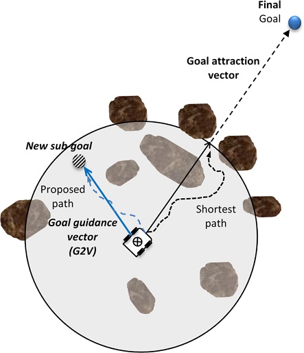
Fig. 1(a) shows a typical case of applying the shortest path algorithm to a simple environment. At first, the robot’s trajectory is a straight line between the robot and the goal; the robot then goes around the wall of the obstacle to take the shortest path to the goal. In this case, the shortest path algorithm is highly effective. However, Fig. 1(b) shows how this algorithm can fail when the robot is trapped by an obstacle in trying to follow the shortest path in a complex environment, i.e., when obstacles are encountered in the direction of the straight line between the robot and the goal. This case shows that it is not always effective for the robot to move in the direction of the final goal throughout the driving process. In the G2V algorithm strategy, a new sub-goal is determined using the end-point of the goal guidance vector in the laser measurement sensor (LMS) range. The new sub-goal is created at the location that represents the minimum risk by using obstacle deviation and pattern information in the HCF. A G2V guide is determined, where the starting point of the vector is the current location of the robot, and the end-point of the vector is the location of the sub-goal.
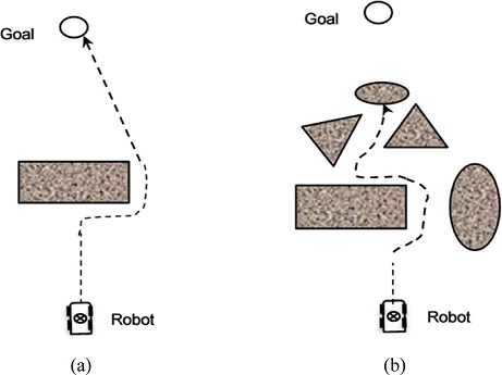
Illustration of the shortest path algorithm for (a) A simple environment and (b) A complex environment around the straight path between the robot and the goal
The G2V is used within the obstacle avoidance algorithm to guide the robot in the direction of minimum risk to avoid colliding with obstacles, as shown in Fig. 2. Fig. 2 shows that if the robot uses the shortest path algorithm in such an environment, the robot will fail to drive because of the numerous obstacles in the path of the goal attraction vector. The HCF used to determine the G2V is calculated by considering the location and scale of each obstacle and enables the robot to drive while avoiding nearby obstacles. The hazard cost function ensures that the robot avoids high risk areas, while remaining aligned with the goal. However, the shortest path remains fixed in the direction of the goal attraction vector regardless of the changes in the environment.
2.2 The Algorithm Model
An occupancy grid map for the positions of the robot and the obstacles is used in the algorithm. An occupancy grid is a M × N matrix that represents a 2-dimensional space. The cells containing zeros are free space where the robot can move, and the cells containing ones are obstacles into which the robot cannot move. The robot is represented by (x, y)∈R2 and the drivable regions and the obstacles are represented as polygons, each of which comprises lists of vertices or edges.26
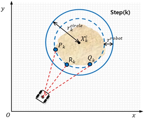
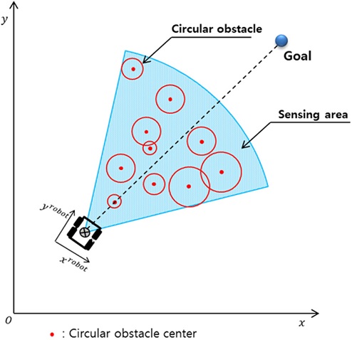
An obstacle is modelled as a circle using three detection points from a laser measurement system (LMS), as shown in Fig. 3. The LMS obtains information for three points (Pk, Qk, Rk) that are detected for an obstacle within sensing range. These three points are used to construct a unique circle centered at Xkc with a radius rkcircle using the equations in Table 1.25 The robot is treated as a point mass; therefore, a virtual circular obstacle can be created using the radius of the circumscribed circle (rrobot) of the robot. These circular obstacles are filled with ones and recorded in the occupancy grid map.
2.3 Using the Hazard Cost Function (HCF) to Formulate the G2V
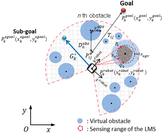
The G2V uses the sub-goal (Pksgoal) as an end-point and the current robot location (Pkrobot) as a starting point in the grid map, as shown in Eqs. (1), (2) and Fig. 4.
| (1) |
| (2) |
The continuously changing location of the sub-goal (Pksgoal) in an unknown environment is a key feature of the developed algorithm that is determined from the hazard cost function (HCF, S). This function is calculated for each grid cell within sensing range. The sub-goal with the lowest grid cell cost is chosen. The cost function S has three terms, as shown in Eq. (3).
| (3) |
| (4) |
The obstacle function (Hij) is designed to minimize the risk from the obstacles in an unknown environment and to calculate the obstacle density in each grid cell within sensing range. A grid cell with a high obstacle density results in a high cost and is considered to be a dangerous point. The obstacle density is a function of the distance between each virtual circular obstacle (Dnobs) and each grid cell (), and the radius of the virtual circular obstacle (rnobs) that is nearest to each grid cell, as shown in Eqs. (6) and (7). Crowding many obstacles into a small area results in a high calculated obstacle density that is difficult for the robot to drive through, as shown in Fig. 5. is the normalized obstacle function. The parameters ε and η tune the value of this function.
| (5) |
where n = n th obstacle
| (6) |
where M= number of the grid cells within sensing range
| (7) |
where N = total obstacles
| (8) |
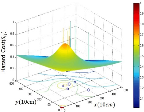
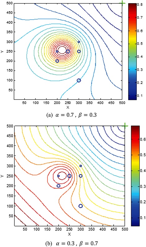
Hazard cost of an environment containing arbitrary obstacles: Six obstacles (shown as blue circles) were used in a 500 × 500 (cm) grid map. The primary contribution to the HCF potential comes from the interior of the dense obstacles
The goal-oriented function (Tij) that maintains the orientation of the robot toward the final goal is found by calculating the Euclidean distance between each cell () and the final goal (Pgoal): is the normalized goal-oriented function.
| (9) |
| (10) |
The penalty constant (ξ) equals the uncertain area that is ruled out in the local grid map-sensing range of the LMS.
| (11) |
The detectable rear obstacles and the sensing area outside the LMS range in a M × N matrix make up a considerable uncertain area for safe driving. The penalty constant serves as an artificial constraint on the sub-goal selection. The weighting factors (α, β) in the HCF serve to tune the motion of the robot. For instance, a large value of α results in the robot moving in the direction that offers the minimum risk, and an attractive goal corresponds to a large β value. Thus, tuning the weighting factors in the HCF affects robot motion. Fig. 6 shows the effect of varying the weighting factors (α, β) in the HCF. The value of α is increased by using five obstacles in a concentrated region. To avoid a high concentration of obstacles, increasing α creates a G2V in another direction.
3. Reactive Fuzzy Control of the Weighting Factor in the HCF
In practice, reactive control of the developed weighting factors corresponds to a compromise between the minimum risk and the attractive goal. Fuzzy-Logic-based control is applied to realize a reactive strategy for the robot, because this type of control is sufficiently fast and effective to react in real time to an unknown environment. The weighting factor is formulated using fuzzy rules. The fuzzy input is the pattern formula of the center of the circular obstacles that are detected by LMS. The fuzzy output is the weighting factor α, and β is determined from α + β = 1.
3.1 Estimating the Obstacle Pattern Formula for the Fuzzy Input
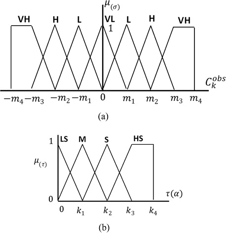
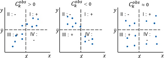
The fuzzy input is represented by a linguistic fuzzy set with four members {VL, L, H, VH} with the membership function shown in Fig. 7(a) and is derived from simple numerical measures for estimating the pattern formula for the location of the obstacles within sensing range, as shown in Fig. 8. The numerical measures are estimated by calculating the correlation coefficient from Eqs. (12)-(14).27 In robot driving, it is important to determine whether the pattern formed by the obstacles is complex or simple. The center of the obstacle (xi, yi) as detected by LMS is considered to be a scatterplot in the 2D plane. The scatterplot can have a linear or nonlinear pattern, as shown in Fig. 9. For instance, when a straight line can be fit through the data points, the obstacle pattern is linear, and the obstacles are distributed regularly making it less dangerous to drive. However, an irregular distribution corresponds to a relatively dangerous distribution of obstacles.
| (12) |
| (13) |
| (14) |
A correlation coefficient can be used to describe each of the variables xi and yi individually using a descriptive measure such as the standard deviation. The correlation coefficient is denoted by Ckobs and is defined in Eq. (12). The quantities Skx and Sky are the standard deviations for the variables xi and yi, respectively, and Skxy is the covariance between xi and yi is defined in Eqs. (13) and (14). The value of the correlation coefficient (Ckobs) ranges between -1 and 1: when Ckobs is close to 1 or -1, a stronger pattern indicates a higher linearity in the data. In contrast, when Ckobs is close to 0, the data points are scattered across all four areas and is there is no obvious pattern, as shown in Fig. 9.
3.2 Fuzzy Output and Rules for Determining the Weighting Factors
The weighting factor α of the HCF is represented by a linguistic fuzzy set with four members {LS, M, S, HS}, with the membership function shown in Fig. 7(b), and is derived from the sets of rules given below.
- If Ckobs is VL, THEN α is HS.
- If Ckobs is L, THEN α is S.
- If Ckobs is H, THEN α is M.
- If Ckobs is VH, THEN α is L
For instance, the robot detects obstacles using the LMS, records the information on the circular obstacles in the grid map and calculates Ckobs to estimate the pattern formula of the obstacles. If Ckobs is VH, the pattern is complex and dangerous; thus, α is increased to minimize the risk, and HS is selected.
However, if few obstacles (Nkobs) are within sensing range, it is not meaningful to calculate Ckobs. In this case, it is necessary to use the following rules. Using the rules given above, α always has a fixed small value for a low obstacle density, which creates a G2V in a direction that rapidly drives the robot toward the final goal.
- If Nkobs is ZERO or < n, THEN α is LS.
- If Nkobs is ≥ n, THEN α is estimated by Ckobs.
4. Perfrmance Analysis based on Simulation
4.1 Virtual Tangential Vector (VTV) Algorithm
The performance of reactive navigation algorithms, such as VFH, etc., can be enhanced by applying the G2V algorithm for obstacle avoidance. As previously mentioned, the G2V algorithm enables the robot to determine the optimal direction while avoiding obstacles, which can increase the success probability of achieving the final goal. Thus, the performance of the reactive navigation algorithm using the shortest path method is significantly improved by combining it with the G2V algorithm: in this method, the robot moves in the closest direction to the final goal in an open area (i.e., where there are no obstacles).
To verify the G2V algorithm, we combine the G2V algorithm with the virtual tangential vector (VTV) algorithm25 in a simulation. The VTV algorithm is a reactive navigation algorithm, which uses the shortest path method with obstacle avoidance. The VTV drives a robot along the tangential direction to a virtual circular obstacle generated in real time. The weighted resultant vector of all the VTVs, the so-called weighted VTV (WVTV), which is defined for multiple obstacles. The WVTV is incorporated into a multi-objective optimization framework: the slope of the VTV can be easily obtained and the final VTV direction toward the goal is determined.
The modified vector field histogram (MVFH) algorithm decomposes the set of 540 directions from the LMS into an obstacle-containing area and an obstacle-free or open area by determining whether the normalized distance between the robot and an obstacle is smaller than a prescribed threshold or not. The middle vector in each open area is then obtained. The vector which makes the smallest angle with the goal attraction vector is selected among all the middle vectors.
4.2 Simulation Model
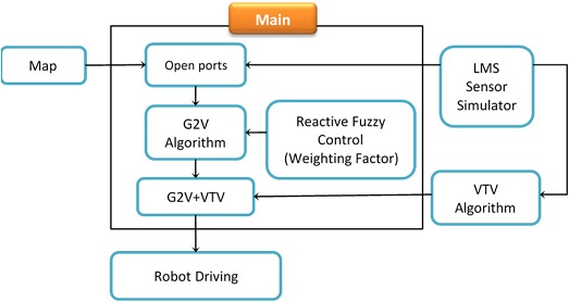
The simulation was performed using a MATLAB program, and an LMS simulator was used with a detection range of 0.1 to 10 m, 270°, and an angular resolution of 0.5°. The LMS was used to measure the distance and the angle between the robot and an obstacle. The robot model was applied to an Ackerman vehicle with front steering with a robot of dimensions 2 (W) × 3 (L) m. The constraints on the robot model in the simulation were a maximum allowable steering angle of 30° and a robot step size of 1.5 m. A global positioning system (GPS) and an inertia measurement unit (IMU) were also used. Fig. 10 is a schematic of the simulation model, and Fig. 11 shows an example of the robot motion using the G2V algorithm.
4.3 Simulation Results and Performance Analysis
In this section, the robot motion is illustrated using several simulations that were conducted for an environment similar to that of related studies. Fig. 12 shows that the G2V that was created for a simple environment of obstacles.
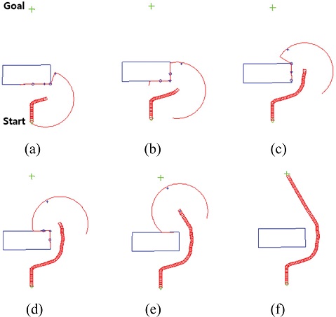
G2V creation in a simple environment of obstacles: starting point (Green circle), final goal (Green cross), G2V end-point (Blue cross), sensing range (Large red circle), and robot motion (Small red circle); weighting factors: α = 0.6, β = 0.4 (Fixed)
The end-point (Which is Shown as a Blue Cross) of the G2V was located to the right side of the obstacle in the sensing range (Which is Shown as a Non-Continuous Red Circle). The end-point was not close to the obstacle and was too far from robot, as shown in Figs. 12(a)-12(c). When the robot was on the right side of the obstacle, as shown in Figs. 12(d)-12(f), the end-point of the G2V was in the direction of the shortest distance to the final goal because there were no obstacles.
Fig. 13 shows the advantages that the developed algorithm offers over the VTV algorithm. When the VTV algorithm was used by itself, the robot moved along the A-B-C path between the obstacles to reach the goal in the shortest distance, as shown in Fig. 13(a). In the C-D path, the robot was trapped by three obstacles, which was similar to being trapped in a local minimum, because the robot moved the shortest distance in the diagonal direction to reach the goal.
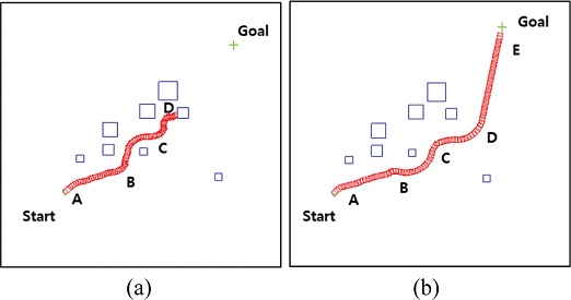
G2V results: (a) Using only the VTV algorithm and (b) Using the proposed algorithm with fuzzy control of the weighting factors
However, using the developed algorithm enabled the robot to avoid the obstacle traps on the C-D path, as shown in Fig. 13(b). The area to the left of the sensing range of the robot had a high HCF cost; therefore, the obstacle avoidance mechanism caused the robot to follow a detour-like path away from the obstacles. Thus, the robot moved along the curved path A-B-C-D-E. Note that the robot turned around the points B, C and D.
Fig. 14 shows the simulation results that were obtained using fuzzy reactive control for the weighting factors in a complex environment made by many circle obstacles. The robot was initially surrounded by scattered obstacles (A-B), resulting in high values for the HCF cost and the weighting factor α. When the robot steered to the left, α changed progressively to a low value (HS-LS, 0.85-0.60) as the obstacle pattern became simple relative to the robot coordinates. The complex obstacle pattern on the B-C path resulted in a fuzzy output of HS for α again. Then, α decreased the fuzzy output from HS to LS progressively toward the final destination, and the robot successfully reached the destination.
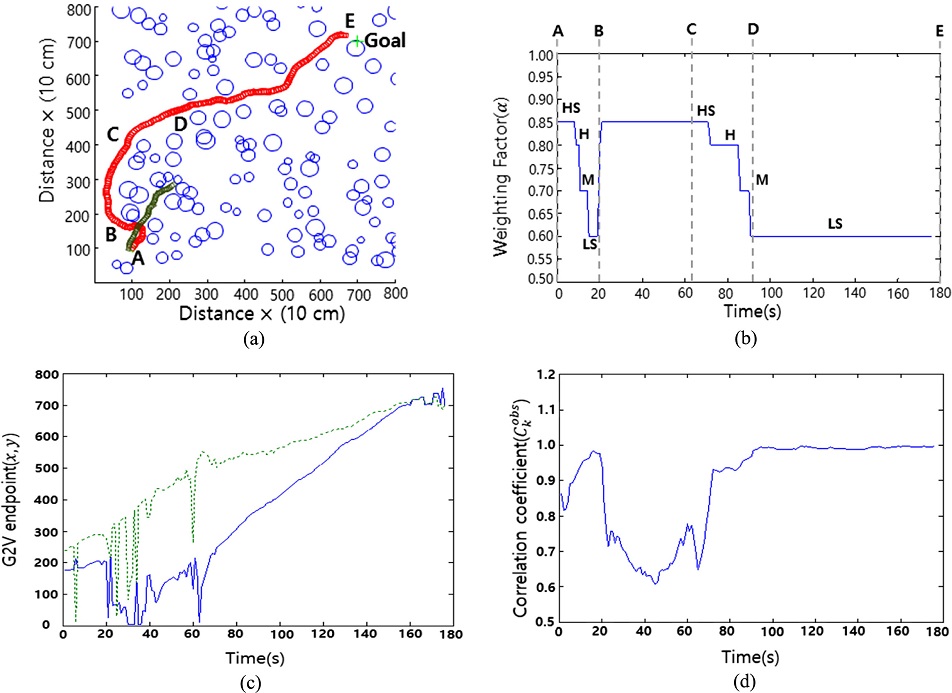
Simulation results for fuzzy reactive control in a complex environment: (a) Robot motion (Red: G2V algorithm, Green: VFH algorithm), (b) The variations in the weighting factor (α) with each step, (c) Coordinates of the G2V end-point (Blue: x, Green: y) and (d) Variation in the correlation coefficient (Ckobs) with each step; the coordinate axes were set at an artificial wall
This result shows that the proposed algorithm offered the advantage that the robot responded effectively in many obstacles. For instance, the robot’s motion along the A-B-C path showed that a complex environment of obstacles could be avoided to minimize risk. The robot’s motion along the C-D-E paths showed that the robot moved efficiently through a short distance toward the goal. However, when the VFH algorithm was used by itself, the robot was trapped by dense obstacle as shown in Fig. 13(a). Finally, 500 times of the simulation results, a success ratio of the proposed algorithm is higher than the VFH and A* algorithm, as shown in Table 2. The position of obstacles was randomly changed for each simulation. VHF algorithm use only bits of the given information to determine a guidance direction by using a histogram of the measured obstacle density distribution. A* algorithm does not consider the steering motion and safety factors of the robot. Therefore, the success rate of the VHF and A* algorithm is lower than that of the G2V algorithm.
We also tested the developed algorithm in a narrow alley and a U-Shaped environment. Fig. 15(a) shows that the robot moved into the middle of the narrow alley relatively safely. The shortest distance algorithm would have caused the robot to move along a wall edge in the direction of the closest goal. Thus, the developed algorithm performed better than the shortest distance algorithm for this environment.
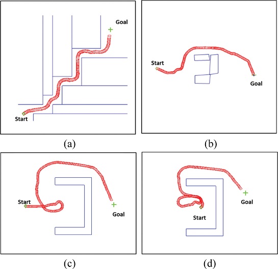
Simulation results for a narrow alley and a U-shaped environment: (a) A narrow alley, (b) The U-shaped region was smaller than the sensing range (Entrance width: 10 m), (c) The U-shaped region was larger than the sensing range (Entrance width: 10 m, starting from the outer edge) and (d) The U-shaped region was larger than the sensing range (Starting from the inner edge), Sensing range: 15 m
From Figs. 15(b) to 15(d) show the simulation results for the U-Shaped obstacle. Fig. 15(b) shows that the obstacle was smaller than the sensing range (15 m), such that the robot detoured to the outside of the U-Shaped obstacle, because the inside of the U-Shaped obstacle represented a high HCF cost.
Fig. 15(c) shows the robot motion for a U-Shaped obstacle that was larger than the sensing range. The robot initially moved into the U-Shaped region, moved back when the obstacle was detected, and detoured safely around the obstacle.
Fig. 15(d) shows the simulation result when the robot started from the inner side of the obstacle. The robot initially moved toward the open area of the U-Shaped region and then moved again toward the inside of the U-Shaped region, because the obstacle was not detected when the robot escaped from the U-Shaped region. The robot then escaped from the U-Shaped region. In this case, the robot’s behavior was inefficient.
5. Conclusion
In this paper, we developed a new reactive navigation algorithm known as the G2V algorithm to minimize the risk within sensing range. The G2V algorithm was designed to improve the performance of the reactive navigation algorithm, which was used to determine the optimal direction that offers the minimum risk, i.e., a HCF function that accounted for the scale and location of the obstacles within the sensing range of the robot was used. We also applied real-time fuzzy reactive control to determine the weighting factors for the HCF in an unknown environment. Simulation results using MATLAB showed that the advantage offered by the developed algorithm was that the robot responded effectively to changes in the environment.
The developed algorithm also showed that the robot detoured safely around the obstacle in a U-Shaped region. Despite the advantages offered by the developed algorithm, inefficient motion was observed in some environments, such as starting from the inside of a U-Shaped region: these inefficiencies should be improved upon. Future work should therefore involve improving the developed algorithm to eliminate inefficient robot behavior in various specific environments.
REFERENCES
-
Khatib, O., “Real-Time Obstacle Avoidance for Manipulators and Mobile Robots,” Autonomous Robot Vehicles, Vol. 5, pp. 396-404, 1986.
[https://doi.org/10.1007/978-1-4613-8997-2_29]

-
Borenstein, J. and Koren, Y., “Real-Time Obstacle Avoidance for Fast Mobile Robots,” IEEE Transactions on Systems, Man, and Cybernetics, Vol. 19, No. 5, pp. 1179-1187, 1989.
[https://doi.org/10.1109/21.44033]

-
Borenstein, J. and Koren, Y., “The Vector Field Histogram-Fast Obstacle Avoidance for Mobile Robots,” IEEE Transactions on Robotics and Automation, Vol. 7, No. 3, pp. 278-288, 1991.
[https://doi.org/10.1109/70.88137]

- Simmons, R., “The Curvature-Velocity Method for Local Obstacle Avoidance,” Proc. of the IEEE International Conference on Robotics and Automation, pp. 3375-3382, 1996.
-
Fox, D., Burgard, W., and Thrun, S., “The Dynamic Window Approach to Collision Avoidance,” IEEE Robotics & Automation Magazine, Vol. 4, No. 1, pp. 23-33, 1997.
[https://doi.org/10.1109/100.580977]

-
Fernández, J. L., Sanz, R., Benayas, J., and Diéguez, A. R., “Improving Collision Avoidance for Mobile Robots in Partially Known Environments: The Beam Curvature Method,” Robotics and Autonomous Systems, Vol. 46, No. 4, pp. 205-219, 2004.
[https://doi.org/10.1016/j.robot.2004.02.004]

-
Shi, C., Wang, Y., and Yang, J., “A Local Obstacle Avoidance Method for Mobile Robots in Partially Known Environment,” Robotics and Autonomous Systems, Vol. 58, No. 5, pp. 425-434, 2010.
[https://doi.org/10.1016/j.robot.2010.02.005]

-
Molinos, E., Llamazares, Á., Ocaña, M., and Herranz, F., “Dynamic Obstacle Avoidance based on Curvature Arcs,” Proc. of the IEEE/SICE International Symposium on System Integration, pp. 186-191, 2014.
[https://doi.org/10.1109/SII.2014.7028035]

-
Minguez, J. and Montano, L., “Nearness Diagram (ND) Navigation: Collision Avoidance in Troublesome Scenarios,” IEEE Transactions on Robotics and Automation, Vol. 20, No. 1, pp. 45-59, 2004.
[https://doi.org/10.1109/TRA.2003.820849]

-
Mujahad, M., Fischer, D., Mertsching, B., and Jaddu, H., “Closest Gap Based (CG) Reactive Obstacle Avoidance Navigation for Highly Cluttered Environments,” Proc. of the IEEE/RSJ International Conference on Intelligent Robots and Systems, pp. 1805-1812, 2010.
[https://doi.org/10.1109/IROS.2010.5649736]

-
Lumelsky, V. J. and Stepanov, A. A., “Path-Planning Strategies for a Point Mobile Automaton Moving Amidst Unknown Obstacles of Arbitrary Shape,” Algorithmica, Vol. 2, Nos. 1-4, pp. 403-430, 1987.
[https://doi.org/10.1007/BF01840369]

-
Lumelsky, V. J. and Skewis, T., “Incorporating Range Sensing in the Robot Navigation Function,” IEEE Transactions on Systems, Man, and Cybernetics, Vol. 20, No. 5, pp. 1058-1069, 1990.
[https://doi.org/10.1109/21.59969]

-
Kamon, I., Rimon, E., and Rivlin, E., “Tangentbug: A Range-Sensor-Based Navigation Algorithm,” The International Journal of Robotics Research, Vol. 17, No. 9, pp. 934-953, 1998.
[https://doi.org/10.1177/027836499801700903]

-
Laubach, S. and Burdick, J., “Roverbug: Long Range Navigation for Mars Rovers,” Experimental Robotics VI, pp. 339-348, 2000.
[https://doi.org/10.1007/BFb0119412]

-
Kamon, I., Rimon, E., and Rivlin, E., “Range-Sensor-Based Navigation in Three-Dimensional Polyhedral Environments,” The International Journal of Robotics Research, Vol. 20, No. 1, pp. 6-25, 2001.
[https://doi.org/10.1177/02783640122067246]

-
Taylor, K. and LaValle, S. M., “I-Bug: An Intensity-Based Bug Algorithm,” Proc. of the IEEE International Conference on Robotics and Automation, pp. 3981-3986, 2009.
[https://doi.org/10.1109/ROBOT.2009.5152728]

-
Kamon, I. and Rivlin, E., “Sensory-Based Motion Planning with Global Proofs,” IEEE Transactions on Robotics and Automation, Vol. 13, No. 6, pp. 814-822, 1997.
[https://doi.org/10.1109/70.650160]

-
Lim, J. H. and Choo, D. W., “Sonar Based Systematic Exploration Method for an Autonomous Mobile Robot Operating in an Unknown Environment,” Robotica, Vol. 16, No. 6, pp. 659-667, 1998.
[https://doi.org/10.1017/S0263574798000587]

-
Krishna, K. M. and Kalra, P. K., “Perception and Remembrance of the Environment during Real-Time Navigation of a Mobile Robot,” Robotics and Autonomous Systems, Vol. 37, No. 1, pp. 25-51, 2001.
[https://doi.org/10.1016/S0921-8890(01)00150-6]

-
Maaref, H. and Barret, C., “Sensor-Based Navigation of a Mobile Robot in an Indoor Environment,” Robotics and Autonomous Systems, Vol. 38, No. 1, pp. 1-18, 2002.
[https://doi.org/10.1016/S0921-8890(01)00165-8]

- Xu, W., Tso, S., and Lu, Z., “A Virtual Target Approach for Resolving the Limit Cycle Problem in Navigation of a Fuzzy Behaviour-Based Mobile Robot,” Proc. of the IEEE/RSJ International Conference on Intelligent Robots and Systems. Innovations in Theory, Practice and Applications, pp. 44-49, 1998.
-
Xu, W. and Tso, S. K., “Sensor-Based Fuzzy Reactive Navigation of a Mobile Robot through Local Target Switching,” IEEE Transactions on Systems, Man, and Cybernetics, Part C (Applications and Reviews), Vol. 29, No. 3, pp. 451-459, 1999.
[https://doi.org/10.1109/5326.777079]

- Pin, F. G. and Bender, S. R., “Adding Memory Processing Behaviors to the Fuzzy Behaviorist Approach (FBA): Resolving Limit Cycle Problems in Autonomous Mobile Robot Navigation,” Intelligent Automation & Soft Computing, Vol. 5, No. 1, pp. 31-41, 1999.
-
Wang, M. and Liu, J. N., “Fuzzy Logic-Based Real-Time Robot Navigation in Unknown Environment with Dead Ends,” Robotics and Autonomous Systems, Vol. 56, No. 7, pp. 625-643, 2008.
[https://doi.org/10.1016/j.robot.2007.10.002]

-
Kwak, K. W., Kim, K. S., and Kim, S., “Weighted Virtual Tangential Vector Algorithm for Local Path Planning of Mobile Robots,” Electronics Letters, Vol. 49, No. 4, pp. 255-256, 2013.
[https://doi.org/10.1049/el.2012.3893]

-
Corke, P., “Robotics, Vision and Control,” Springer, pp. 87-105, 2011.
[https://doi.org/10.1007/978-3-642-20144-8_5]

- Mendenhall, W., Beaver, R. J., and Beaver, B. M., “Introduction to Probability and Statistics,” Cengage Learning, 2012.
-
Filliat, D. and Meyer, J. A., “Map-Based Navigation in Mobile Robots: I. A Review of Localization Strategies,” Cognitive Systems Research, Vol. 4, No. 4, pp. 243-282, 2003.
[https://doi.org/10.1016/S1389-0417(03)00008-1]

-
Meyer, J. A. and Filliat, D., “Map-Based Navigation in Mobile Robots: II. A Review of Map-Learning and Path-Planning Strategies,” Cognitive Systems Research, Vol. 4, No. 4, pp. 283-317, 2003.
[https://doi.org/10.1016/S1389-0417(03)00007-X]

-
Minguez, J. and Montano, L., “Nearness Diagram (ND) Navigation: Collision Avoidance in Troublesome Scenarios,” IEEE Transactions on Robotics and Automation, Vol. 20, No. 1, pp. 45-59, 2004.
[https://doi.org/10.1109/TRA.2003.820849]

-
Borenstein, J. and Koren, Y., “Histogramic in-Motion Mapping for Mobile Robot Obstacle Avoidance,” IEEE Transactions on Robotics and Automation, Vol. 7, No. 4, pp. 535-539, 1991.
[https://doi.org/10.1109/70.86083]

- Brock, O. and Khatib, O., “High-Speed Navigation Using the Global Dynamic Window Approach,” Proc. of the IEEE International Conference on Robotics and Automation, pp. 341-346, 1999.
- Ulrich, I. and Borenstein, J., “VFH+: Reliable Obstacle Avoidance for Fast Mobile Robots,” Proc. of the IEEE International Conference on Robotics and Automation, pp. 1572-1577, 1998.
- Koren, Y. and Borenstein, J., “Potential Field Methods and their Inherent Limitations for Mobile Robot Navigation,” Proc. of the IEEE Conference on Robotics and Automation, pp. 1398-1404, 1991.
-
Motlagh, O., Tang, S. H., Ismail, N., and Ramli, A. R., “An Expert Fuzzy Cognitive Map for Reactive Navigation of Mobile Robots,” Fuzzy Sets and Systems, Vol. 201, pp. 105-121, 2012.
[https://doi.org/10.1016/j.fss.2011.12.013]

- Simmons, R., “The Curvature-Velocity Method for Local Obstacle Avoidance,” Proc. of the IEEE International Conference on Robotics and automation, pp. 3375-3382, 1996.
-
Jeong, H. K., Choi, K. H., Kim, S. H., and Kwak, Y. K., “Driving Mode Decision in the Obstacle Negotiation of a Variable Single-Tracked Robot,” Advanced Robotics, Vol. 22, Nos. 13-14, pp. 1421-1438, 2008.
[https://doi.org/10.1163/156855308X360497]

-
Mujahed, M., Fischer, D., and Mertsching, B., “Tangential Gap Flow (TGF) Navigation: A New Reactive Obstacle Avoidance Approach for Highly Cluttered Environments,” Robotics and Autonomous Systems, Vol. 84, pp. 15-30, 2016.
[https://doi.org/10.1016/j.robot.2016.07.001]

-
Patle, B., Pandey, A., Parhi, D., and Jagadeesh, A., “A Review: On Path Planning Strategies for Navigation of Mobile Robot,” Defence Technology, Vol. 15, No. 4, pp. 582-606, 2019.
[https://doi.org/10.1016/j.dt.2019.04.011]

-
Gonzalez, R., Kloetzer, M., and Mahulea, C., “Comparative Study of Trajectories Resulted from Cell Decomposition Path Planning Approaches,” Proc. of the 21st International Conference on System Theory, Control and Computing, pp. 49-54, 2017.
[https://doi.org/10.1109/ICSTCC.2017.8107010]

-
Raja, R., Dutta, A., and Venkatesh, K., “New Potential Field Method for Rough Terrain Path Planning Using Genetic Algorithm for a 6-Wheel Rover,” Robotics and Autonomous Systems, Vol. 72, pp. 295-306, 2015.
[https://doi.org/10.1016/j.robot.2015.06.002]

-
Patle, B., Parhi, D., Jagadeesh, A., and Kashyap, S. K., “Matrix-Binary Codes Based Genetic Algorithm for Path Planning of Mobile Robot,” Computers & Electrical Engineering, Vol. 67, pp. 708-728, 2018.
[https://doi.org/10.1016/j.compeleceng.2017.12.011]

-
Al Mutib, K., Mattar, E., and Alsulaiman, M., “Implementation of Fuzzy Decision Based Mobile Robot Navigation Using Stereo Vision,” Procedia Computer Science, Vol. 62, pp. 143-150, 2015.
[https://doi.org/10.1016/j.procs.2015.08.427]

-
Patle, B., Parhi, D., Jagadeesh, A., and Kashyap, S. K., “Probabilistic Fuzzy Controller Based Robotics Path Decision Theory,” World Journal of Engineering, Vol. 13, pp. 181-192, 2016.
[https://doi.org/10.1108/WJE-04-2016-024]


Ph.D. in the Department of Mechanical Engineering, Korea Advanced Institute Science and Technology (KAIST). His research interest is autonomous robot.
E-mail: choiha99@kaist.ac.kr

Professor at the Department of Mechanical Engineering, Korea Advanced Institute Science and Technology (KAIST). His research interest is Bio-inspired robot.
E-mail: soohyun@kaist.ac.kr

