Quantitative Metallographic Analysis of GCr15 Microstructure Using Mask R-CNN

1. Introduction

Quantitative metallography is a very important method in materials analysis. It highlights the relationship between processes and microstructures as well as their associated mechanical and physical properties. One other importance of quantitative metallography is its ability to supply first-hand data which is useful in establishing a logical-mathematical representation and the understanding of the mechanical properties of the metals. These processes are very instrumental in improving existing materials and also in the development of new ones.¹ Research and development departments consider quantitative microstructure characterization as an important procedure in the quality control of materials and products.¹⁴ An analysis of the composition of the internal and metallographic structures makes it easier to understand. This is done through using an optical metallographic microscope or using an electron microscope and other analytical instruments to analyze the characteristics of the material. This shows the important role metallographic analysis plays in establishing the quantitative relationship between the structure and its performance.^3,4 GCr15 bearing steel is used in the manufacturing of rolling bearings as well as rolling rings. Due to its functionality, the microstructure and performance of bearing steel are often researched and studied.^15-18

Rolling bearings like GCr15 bearing steel are used in different fields of life and most importantly in the advancement of science and technology. The use of this metal has inspired researches and contributed significantly to the progress made in advanced vehicles, high-speed railways and other technologies in the aviation industry. However, meeting the demands of this rapidly developing industry requires improvement in its mechanical properties to meet the demands. In our research, our task was to locate and segment the carbide particles present within the GCr15 microstructure, to use a less tedious approach as compared to the methods used by Zhao et al. (2016).^1,4,6

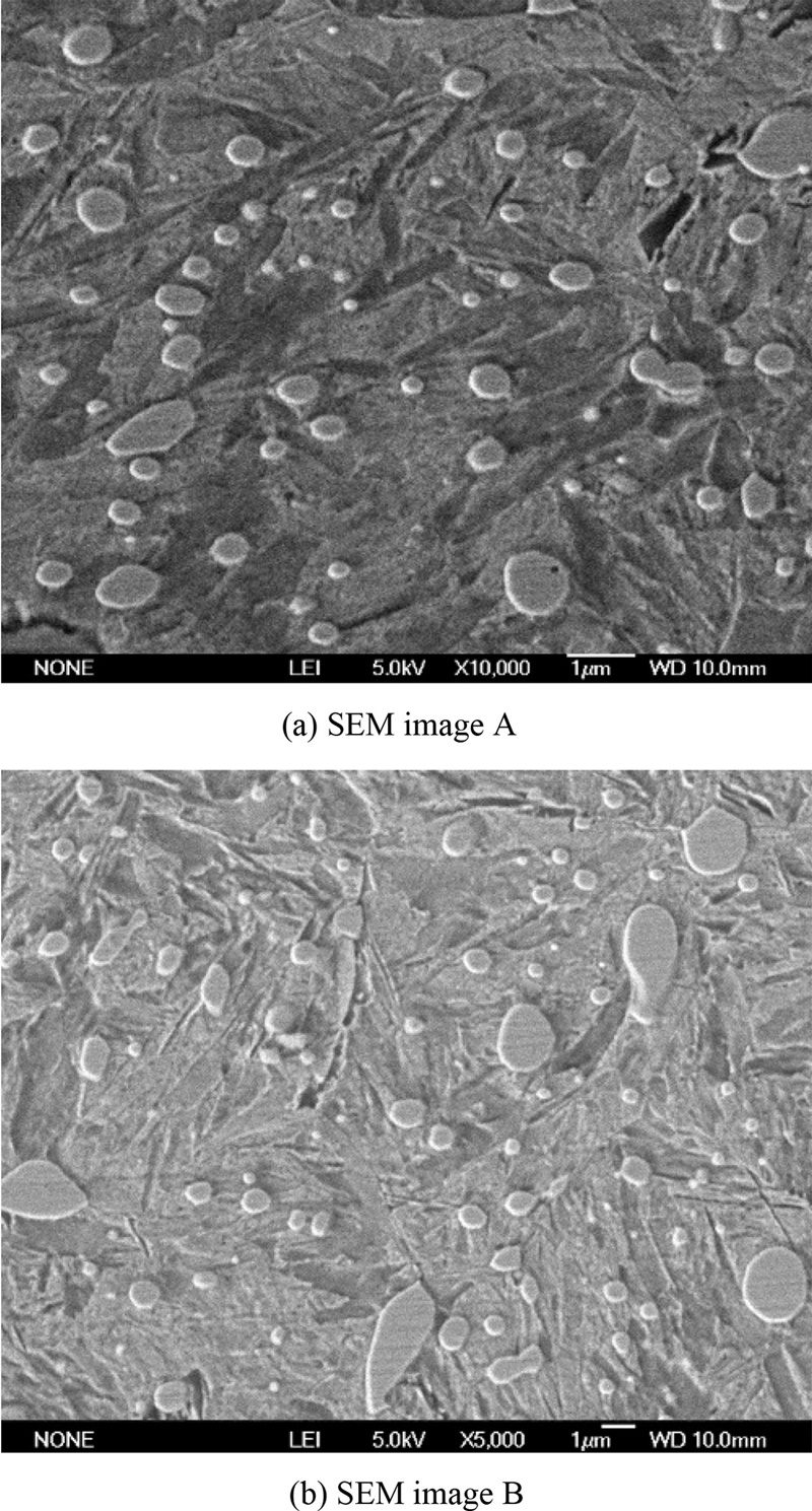
The image of GCr15 microstructure is quite delicate because its foreground and background are basically of the same color and proved to be challenging during processing. The edges of the holes in the image have similar pixel values as the boundaries of the carbide particles.⁶ In the experiment by Zhao et al. (2016), the image analysis was done by cropping the image into segments before processing the image using the traditional method of image segmentation which proved to be very slow and challenging.⁶ In our case, we experimented using the Mask R-CNN approach, a branch of CNN. It was a very effective and an efficient method in detecting the carbide particles without cropping the image into sections.

Convolutional neural networks (CNN) are a class of deep learning neural networks and represent a tremendous breakthrough in image recognition and serves as an efficient learning method for hierarchical features from large datasets. Deep learning has emanated as a new field in machine learning and is applied in many image applications. There are key areas where the application of the theory of machine learning and pattern recognition are utilized. Image classification for instance has been one of the most significant topics in the area of computer vision and computer learning. Examples of image applications include facial recognition, car identification, signature authentication and many others.^2,5,25-27

The Mask R-CNN method involves the addition of segmentation masks on the individual region of interest (ROI) to the image under study. The masked section is a pixel-to-pixel segmentation of each ROI by using Fully Convolutional Network. The algorithms of Mask R-CNN are designed to achieve object detection, localization and instance segmentation of the images. It combines Faster RCNN and FCN, introduces ROI-Align to preserve the spatial orientation of features to prevent data loss. Our image; SEM image of the GCr15 microstructure has very little difference between the background and the foreground, which makes it quite challenging to process using the traditional method of segmentation, however, the process of using Mask R-CNN rather proved very effective and easy.⁵

2. Image Acquisition

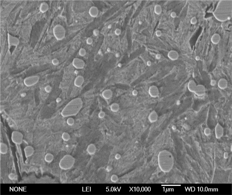
The images of the GCr15 microstructure were acquired after heat tempering and quenching of the GCr15 bearing steel. The metallographic images were obtained by using a JSM-6700 JSM 6700F NT scanning electron microscope (SEM). The Fig. 1 is an example of the SEM image of the GCr15 microstructure of size 1280 × 1024 pixels.⁶

Fig. 1

SEM image of the GCr15 Microstructure, JSM-6700 SEM (1280 × 1024 pixels)6 (Adapted from Ref. 6 on the basis of OA)

3. Method

The Mask R-CNN method is built on Faster R-CNN and was tested on the coco dataset. It also proved efficient on the ResNet-50 and ResNet-101 but better on ResNet-101.⁵ However, some of the analysis we performed required that we import modules like NumPy to help with the blob count, perimeter and area of the blobs. Some components of Mask R-CNN and modules we used to execute our task include:

NumPy, it is a python extension module. We imported this module into our Mask R-CNN algorithm, which was available on GitHub by Matterport. We then stored our numerical results as data in a CSV format. NumPy can be described as a basic package for scientific computing with Python. It encompasses things such as an N-dimensional array object, sophisticated (Broadcasting) functions, tools for integrating C/C++ and Fortran code and a useful linear algebra, Fourier transform as well as random number capabilities. The colors expressed in the image are pixels values which are expressed in the form of arrays. Concerning the Mask R-CNN, NumPy was imported to carefully locate the coordinates for the bounding boxes in terms of x and y and around the targeted images as well as in the area of the blob masking within the bounding boxes.²⁰

Faster R-CNN is an object detection architecture which comprises convolution layers, regional proposal network (RPN) and class boundary box prediction by using a fully connected neural network that uses RPN to take inputs and predict object classes and bounding boxes.²¹

ResNet-50 and ResNet-101 are very efficient and substantially deeper residual learning frameworks. These residual networks proved easier to optimize and with a high level of accuracy. This was done by training it on ImageNet classification dataset with a depth of up to 152 layers.²² The Mask R-CNN was able to perform well on ResNet-101 C4 and FPN, however, the results on FPN outperformed C4.⁵

Fig. 2

Scanning electronic microscopic images of the GCr15 microstructure by the JSM 6700F NT instrument

COCO dataset is defined as Common Objects in Context (COCO) dataset. “COCO is large-scale object detection, segmentation, and captioning dataset. COCO has several features: Object segmentation, Recognition in context, Superpixel stuff segmentation, 330 K images (> 200 K labelled), 1.5 million object instances, 80 object categories, 91 stuff categories, 5 captions per image, 250,000 people with keypoints.” This dataset was used in the open-source project for Matterport’s Mask R-CNN.²⁴

2016 COCO challenge was one of the annual COCO competitions organized in 2016. The winners excelled for their brilliant work on instance segmentation.²⁴

Matterport is an open-source developer account for Mask R-CNN on GitHub. It provided the algorithm for Mask R-CNN for object detection as well as instance segmentation on Keras and TensorFlow.¹⁰

The dataset provided by Zhao et al. (2016) on the GCr15 microstructure as used in their research was very small; 8 in total with size 1280 × 1024 pixels. Due to this, we augmented the dataset by generating new images from the existing data. Data augmentation is an important process in image analysis. It helps us to add more data to the existing one most often due to small dataset. Small datasets do generate the problem of overfitting on test images due to generalization problem on the training model but since data augmentation has proven to be very effective in image classification using deep learning it was the right approach. We used the method of the traditional data augmentation processes such as rotation, cropping to 224 × 224 pixel size, zooming, color distortion, flipping input images and introducing other images that look like our primary image and for each image of size N, a new dataset of size 2 N was produced and subsequently increased our dataset to 50 images.⁷

Our new dataset was N = 50; training data = 30, Validation data = 10, Testing data = 10. This was quite limited but we generated very promising results on our test data. In extracting the features of our blobs, we used the VGG Image Annotator software to annotate the blobs in each image, this was done for N = 40, and saved them as JSON files. The VGG Image Annotator saved each image in the form of x and y coordinates in each region during the annotation. As a result, we loaded these files as a “.json” file and thus made it easier for us to train considering that each coordinate of the shape of the blob is an object instance.⁸

3.1 Using Mask R-CNN Model

Mask R-CNN works towards the problem of instance segmentation, the process of detecting each distinct object present in the image. Instance segmentation is a combination of subproblems in an image. These are:

(a) Object detection

(b) Semantic Segmentation

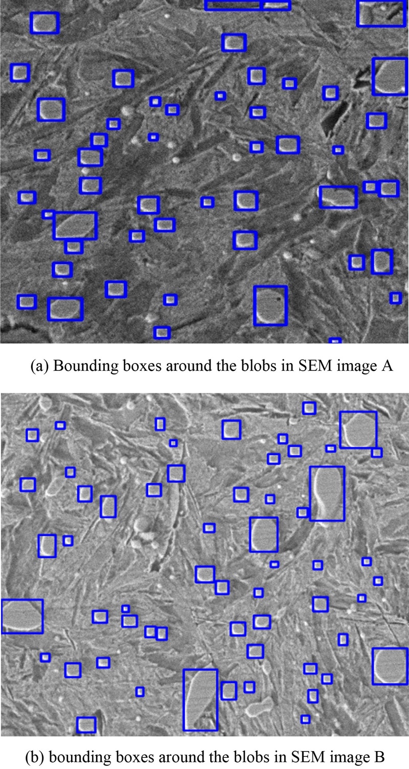
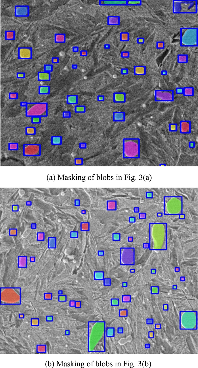
“a” and “b” together form instance segmentation. The bounding boxes generated in Fig. 3 and the masked blobs in Fig. 4 are outputs of semantic segmentation.⁵ Mask-RCNN is simple and flexible. It works by adding a branch for predicting an object mask which is in parallel with the existing branch for bounding box recognition to Faster R-CNN. The Mask-RCNN uses region proposals which are generated via a region proposal network (RPN) present within the Faster R-CNN architecture.^5,21 This approach replaces the ROI-Pooling operation in Faster-RCNN with ROI-Align and generates very accurate instance segmentation masks on the blobs. This was achieved by preserving the spatial orientation of the features followed by adding a network head to produce the desired instance segmentations.^5,9 It was proven that ResNet-101 was effective as a backbone for Mask-RCNN by using a feature pyramid network (FPN). This network proved effective and efficient in terms of accuracy and speed which makes it superior to other methods. Mask R-CNN is designed to train on COCO dataset, a large dataset and proved very successful.^5,23 In this experiment the implementations were done using the algorithms available in GitHub by Matterport which was built using Keras and TensorFlow open-source libraries.^10-12 In our experiment, we used ResNet-101 model as a backbone due to its higher efficiency.^5,9,19 Instead of training the model from scratch, we used transfer learning. We did this by initializing the model weights which was obtained through pretraining on the MS COCO dataset. We subsequently trained only the network heads and fine-tuned some parameters to suit our task. The training was done using AWS P2 instance and generated an accuracy of 99.03%.^9,13

Fig. 3

Locating the blobs using bounding boxes

Fig. 4

Segmentation masks on each blob within the bounding boxes

4. Results and Discussion

We modified the algorithm to first detect the region of interest (ROI); blob areas, by generating only the bounding boxes the blobs. This was achieved by setting the “show mask line” in the Mask R-CNN line of code to “False”. In this case, the results we obtained were without masks, just bounding boxes around the blobs in the image to confirm that our blobs were accurately located.

We then proceeded to mask the blobs by changing the False to True. The results obtained in this process was an improvement on the earlier experiments conducted by Zhao et al. (2016), which includes: image read, gray and image filtering, corrosion and reconstruction of the gray image, image binarization and morphological operations, and finally, area fill and computation. In using the Mask R-CNN method, all we needed to do was run the codes on our SEM images and series of results will be generated; blob number, masked blobs, area and perimeter. We located the carbide particles and achieved over 90% accuracy on a very small dataset.

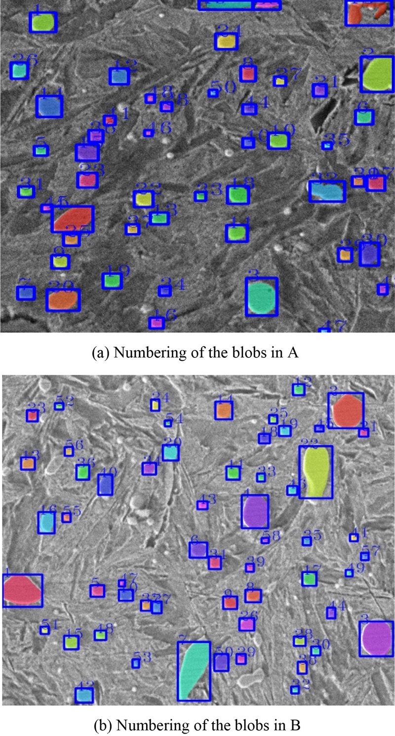
The approach employed by Zhao et al. (2016) is time-consuming and has to be done manually per image. However, with the Mask R-CNN approach, once training is complete and tested successfully, analysis on similar images takes few seconds to complete which is a great advantage that CNNs have over traditional methods of image analysis. The data generated from the images in Fig. 5 are displayed in Tables 1 and 2.

Fig. 5

Using the blob counter to label each blob from i = 1 to the Nth term

Table 1

Blob number, area and perimeter of blobs in SEM image A (Pixel value)

Table 2

Blob number, area and perimeter of Blobs in SEM image A (Pixel value)

Tables 1 and 2 contain the number of blobs for each SEM image and the area and perimeter of the blobs measured in pixels within that image. It can be observed from our images in Figs. 4 and 5 that a vast majority of the carbide particles (Blobs) were captured automatically within the bounding boxes and masked accordingly. For each labelled bounding box, there is a corresponding perimeter and area of the masked blob in that bounding box.

5. Conclusion

These experimental results provided useful and comprehensive data on the quantitative analysis of a complex microstructure of the GCr15 bearing steel using the Mask R-CNN model. This research merges metallographic quantitative analysis and convolutional neural networks (CNNs) to generate data on GCr15 bearing steel microstructure. The results from the Mask R-CNN gave us a comprehensive morphological analysis and with the help of NumPy, we were able to compute the perimeter and the area of the carbide particles masked within the bounding boxes. It has been able to produce high-quality results which contribute to quantitative research. It located most of the carbide particles in the microstructure, masked them and did an efficient numerical operation on each blob by generating quantitative data. With this method, the network was given a vision to identify the target image particles that it was trained to identify. The performance of this model, the Mask R-CNN model proved efficient, effective and serves as great network architecture for semantic segmentation. By knowing and comprehending the microstructural quality of the metal, we can control the properties of the metal, predict its behavior or failure under varying conditions.

Acknowledgments

This work was financially supported by the Key Research and Development Program of Gansu Province (18YF1GA063). We would like to acknowledge “Development and maintenance of VGG Image Annotator (VIA) is supported by EPSRC programme grant Seebibyte: Visual Search for the Era of Big Data (EP/M013774/1)”.

References

• Huang, Y. and Froyen, L., “Quantitative Analysis of Microstructure in Metals with Computer Assistance,” NDT Net, Vol. 6, No. 5, 2001.
• Wang, C. and Xi, Y., “Convolutional Neural Network for Image Classification,” http://www.cs.jhu.edu/~cwang107/files/cnn.pdf, (Accessed 13 APR 2020)
• Dong, Z. L., Wu, K. Y., and Lan, Y. L., “Research on Quantitative Metallographic Analysis for Metallic Materials of Power Grid,” Applied Mechanics and Materials, Vol. 422, pp. 29-34, 2013. [https://doi.org/10.4028/www.scientific.net/AMM.422.29]
• Hatch, J. E., “Aluminium Properties and Physical Metallurgy, Chapter 3: Microstructure of Alloys,” American Society for Metals, pp. 58-104, 2014.
• He, K., Gkioxari, G., Dollár, P., and Girshick, R., “Mask R-CNN,” Proc. of the IEEE International Conference on Computer Vision, pp. 2961-2969, 2017. [https://doi.org/10.1109/ICCV.2017.322]
• Zhao, X., Jin, W. Y., Qi, X. L., and Yan, C. F., “Metallographic Quantitative Analysis for GCr15 by Digital Image Process,” Destech Transactions on Engineering and Technology Research, 2016. [https://doi.org/10.12783/dtetr/icca2016/5991]
• Perez, L. and Wang, J., “The Effectiveness of Data Augmentation in Image Classification Using Deep Learning,” arXiv Preprint: 1712.04621, 2017.
• Dutta, A. and Zisserman, A., “The VGG Image Annotator (VIA),” arXiv Preprint: 1904.10699, 2019.
• Johnson, J. W., “Adapting Mask-RCNN for Automatic Nucleus Segmentation,” arXiv Preprint: 1805.00500, 2018.
• Abdulla, W., “Mask R-CNN for Object Detection and Instance Segmentation on Keras and Tensorflow,” GitHub Repository, 2017, https://github.com/matterport/Mask_RCNN, (Accessed 13 APR 2020)
• Abadi, M., Agarwal, A., Barham, P., Brevdo, E., Chen, Z., et al., “Tensorflow: Large-Scale Machine Learning on Heterogeneous Distributed Systems,” arXiv Preprint: 1603.04467, 2016.
• Keras Documentation, “Keras: The Python Deep Learning Library.” https://keras.io/, (Accessed 13 APR 2020)
• Lin, T. Y., Maire, M., Belongie, S., Hays, J., Perona, P., et al., “Microsoft COCO: Common Objects in Context,” Proc. of the European Conference on Computer Vision, pp. 740-755, 2014. [https://doi.org/10.1007/978-3-319-10602-1_48]
• Wojnar, L., “Application of ASTM Standards in Quantitative Microstructure Evaluation,” Proc. of the Czasopismo Techniczne of Technical Transactions, pp. 41-46, 2016.
• Li, N., Cui, C., Zhao, Y., Zhang, Q., and Bai, L., “Structure and Properties of GCr15 Modified by Multiphase Ceramic Nanoparticles/Fe-C Composite Inoculants,” Materials Science and Engineering: A, Vol. 738, pp. 63-74, 2018. [https://doi.org/10.1016/j.msea.2018.09.074]
• Burrier, H., “ASM Handbook Properties and Selection: Iron Steels and High-Performance Alloys.” ASM International: Materials Park, Vol. 1, pp. 380-388, 1987.
• ASTM STP1327, “Bearing Steels: Into the 21st Century: Inclusion Ratings: Past, Present and Future,” 1998.
• ASTM STP1419, “Bearing Steel Technology,” 2002.
• Vuola, A. O., Akram, S. U., and Kannala, J., “Mask-RCNN and U-Net Ensembled for Nuclei Segmentation,” Proc. of the IEEE 16th International Symposium on Biomedical Imaging, pp. 208-212, 2019. [https://doi.org/10.1109/ISBI.2019.8759574]
• Oliphant, T. E., “A Guide to NumPy,” Trelgol Publishing USA, 2006.
• Ren, S., He, K., Girshick, R., and Sun, J., “ Faster R-CNN: Towards Real-Time Object Detection with Region Proposal Networks,” Proc. of the Advances in Neural Information Processing Systems, pp. 91-99, 2015.
• He, K., Zhang, X., Ren, S., and Sun, J., “Deep Residual Learning for Image Recognition,” Proc. of the IEEE Conference on Computer Vision and Pattern Recognition, pp. 770-778, 2016. [https://doi.org/10.1109/CVPR.2016.90]
• Lin, T. Y., Maire, M., Belongie, S., Hays, J., Perona, P., et al., “Microsoft COCO: Common Objects in Context,” Proc. of the European Conference on Computer Vision, pp. 740-755, 2014. [https://doi.org/10.1007/978-3-319-10602-1_48]
• COCO, Common Objects in Context, “What is COCO?,” http://cocodataset.org/#home, (Accessed 13 APR 2020)
• Zheng, Z., Li, Z., Nagar, A., and Kang, W., “Compact Deep Convolutional Neural Networks for Image Classification,” Proc. of the ICMEW, pp. 1-6, 2015. [https://doi.org/10.1007/978-3-319-24702-1_8]
• Rawat, W. and Wang, Z., “Deep Convolutional Neural Networks for Image Classification: A Comprehensive Review,” Neural Computation, Vol. 29, No. 9, pp. 2352-2449, 2017. [https://doi.org/10.1162/neco_a_00990]
• Deepika, J., Sowmya, V., and Soman, K. P., “Image Classification Using Convolutional Neural Networks,” International Journal of Advancements in Research & Technology, Vol. 3, No. 6, pp. 1661-1668, 2014. [https://doi.org/10.14299/ijser.2014.06.002]