Prediction of Clean-room Air-conditioning Defects Using Deep Learning and a Differential Pressure Sensor

Copyright © The Korean Society for Precision Engineering
This is an Open-Access article distributed under the terms of the Creative Commons Attribution Non-Commercial License (http://creativecommons.org/licenses/by-nc/3.0) which permits unrestricted non-commercial use, distribution, and reproduction in any medium, provided the original work is properly cited.
Abstract
A clean room is used for adjusting the concentration of suspended particles using an air-conditioner. It has a fan-filter unit combining a centrifugal fan and a high-efficiency particulate air filter that purifies the outside air and directly affects its cleanliness. Defects in these systems are typically detected using special sensors for each fault, which can be costly. Therefore, this paper proposes a system for diagnosing defects in the fan-filter unit using a single differential sensor and deep learning. The fan-filter unit is part of the air-conditioning system, and it is usually defective in bearings, filters, and motors. These faults include ball wear, internal bearing contamination, filter contamination, and motor speed changes. Each defect was artificially induced in experiments, and the differential pressure data of each defect was learned using a long short-term memory (LSTM) deep learning algorithm. The results of deep learning experiments generated by randomly mixing data five times were presented using a confusion matrix, and the results showed an accuracy of 87.2±2.60%. Therefore, the possibility of diagnosing defects in the fan-filter unit using a single sensor was confirmed.
Keywords:
Clean room, Fault detection and diagnosis, Deep learning, Fan-filter unit, Air-conditioning equipment, Differential pressure키워드:
클린룸, 결함 검출 및 진단, 딥러닝, 팬-필터유닛, 송풍기, 차압1. Introduction
An abundance of vapor pollutants emitted during semiconductor manufacturing or chemical processes, such as sulfur oxide, nitrogen oxide, ozone, and ammonia, can negatively influence the semiconductor manufacturing environment [1]. Therefore, semiconductor manufacturing and chemical processes are performed in clean rooms, wherein the concentration of suspended particles is controlled. Furthermore, the inflow, generation, and congestion of internal particles are minimized and the temperature, humidity, pressure are controlled [2].
Any variation from the precise environment maintained by the clean room can adversely affect the production and yield of displays and semiconductors produced therein [3]. Problems in clean rooms can be detected by monitoring the vibrations of the air-conditioner as well as variations in the temperature, humidity, and pressure [4-7]. The vibration signal can be measured and monitored using a vibration measurement sensor installed on the motor of the airconditioning system [8], while the temperature, humidity, and pressure can be monitored using a sensor installed inside the clean room[9]. The data signals from the sensors can then be used to diagnose defects using data analysis and AI-based diagnostic methods for experts and non-experts, respectively [10,11].
Defects can occur in various parts of the air-conditioning system, such as the bearings, motors, fans, and high-efficiency particulate air (HEPA) filters. Defects in bearings and motors are mainly diagnosed using vibration sensors [12]. In contrast, the replacement period of the HEPA filter is determined by measuring the differential pressure inside the air-conditioning equipment [13]. Therefore, various sensors are required to diagnose defects in complex clean rooms [14,15]. On the contrary, their usage is limited in terms of cost and data processing capabilities with regards to deep learning.
In this study, the differential pressure of the fan-filter unit in a clean room was monitored and the differential pressure signal caused by defects in the air-conditioner was learned by a deep learning model to confirm the possibility of using a single sensor to diagnose defects in a fan-filter unit.
2. Experiment Setup
2.1 Fan-filter Unit Defects
In this study, the defects of the fan-filter unit were divided into bearing, filter, and motor defects. Bearing defects include bearing element defects due to wear, cracking, and contamination. Bearing wear or cracking can occur on the outer race, ball, and inner race. When defects occur in bearing elements, defects occur in all elements because the elements are interlocked. Thus, we focused on bearing balls where all the elements are engaged.
In this study, to simulate bearing wear, 2 of the 10 ball bearings (NTN 7202B angular ball bearing), were artificially worn to 1 mm depth using a grinder. And, to simulate bearing contamination defect, 0.4 g of aluminum oxide (Al2O3) was injected into bearings (NSK 6202 DDU deep groove ball bearing) [16]. Two kinds of different ball bearings were used in this case. Because there is no sealing in the 7202 bearings. Therefore, the aluminum oxide escapes and does not contaminate the bearing. In contrast, 6202 bearings were not decomposed and were unsuitable for ball-wear bearings. Figs. 1(a) is normal ball, 1(b) is worn ball, 1(c) is normal bearing, 1(d) is contaminated bearing, respectively.
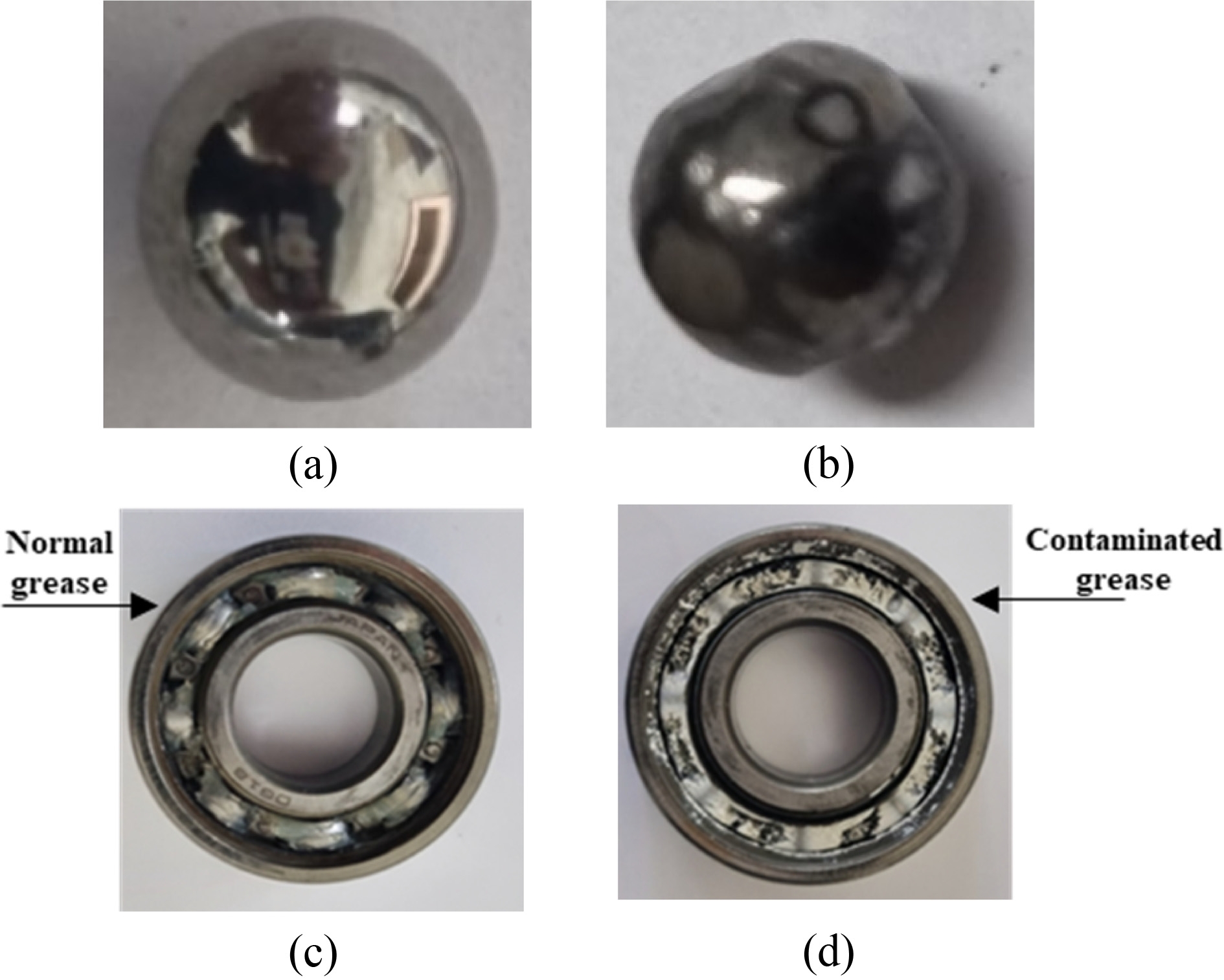
Bearing defects of fan-filter unit: (a) Normal ball, (b) Worn ball, (c) Normal bearing, (d) Contaminated bearing
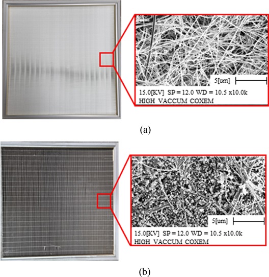
The HEPA filter on the fan-filter unit affects the air purification and must be replaced before the end of its useful life. It the air by catching and retaining particulate, which eventually clogs the filter. The total useful life of the HEPA filter can be determined by measuring the differential pressure inside the air-conditioning equipment. Data on contaminated filters were obtained using filters that had passed their lifespans. Figs. 2(a) and 2(b) show a normal and contaminated filter, respectively, including 1000× magnifications obtained using a scanning electron microscope.
This study simulated a stator winding short circuit, which causes electrical defects in the motor and affects the output speed [17]. The stator winding fails due to an overload, an interlayer short circuit caused by the breakdown of winding insulation, weak insulation, or degradation of the winding, a winding ground where the intersection part is short-circuited, and an instantaneous overvoltage exceeding the internal voltage of the winding. As the number of short-circuited turns of the malfunction increases, the winding resistance also decreases in proportion, thereby increasing the current. Likewise, as the number of short-circuited turns increases, the peak value of the current increases. Induced electromotive force [V] is reduced. Eqs. (1), (2) results in a change in motor RPM, in this experiment, the speed change due to the defect of the motor was simulated by changing the speed from the reference speed of the motor from 1,040 RPM to 1,000 and 1,080 RPM using a speed regulator. K is power, V is voltage, I is current, cos φ is power factor, N is Motor’s speed, T is torque.
| (1) |
| (2) |
2.2 Experiment Configuration
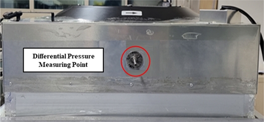
A simple clean room was created to monitor the airconditioning fan-filter unit. A 750 × 800 × 1,000 mm frame was constructed using 50 mm thick aluminum. As the outer walls of a clean room have excellent chemical resistance, a 5 mm thick panel was made using polyvinyl chloride (PVC), which is commonly used in clean rooms [18]. The fan-filter unit was connected to the ceiling of the simple clean room, and the airflow was toward the floor. Square exhaust duct holes (200 × 200 mm) were made on both sides to control the airflow. The size of the fan-filter unit and output wind speed are 576 × 576 × 200 mm and 0.25–0.45 m/s, respectively (Next Technology, NTFFU-575). This experiment was conducted in an indoor environment with no wind of about 33 m2 and the same atmosphere and pressure. The measurement range and response time of the differential pressure sensor are −300-+300 Pa and 10 ms, respectively (Sensys). Figs. 3(a) and 3(b) show the schematic and actual simple clean room, respectively. To check the tendency, the location of measurement of the differential pressure sensor was selected using Solidworks 2019, CFD. The differential pressure sensor measurement position is set as shown in Fig. 4.
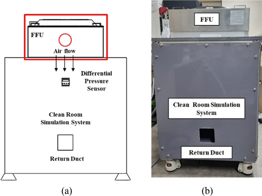
Experiment setup: (a) Configuration of clean room simulation system, (b) Actual configuration of clean room simulation system
3. Experiment
3.1 Ball Bearing Comparison
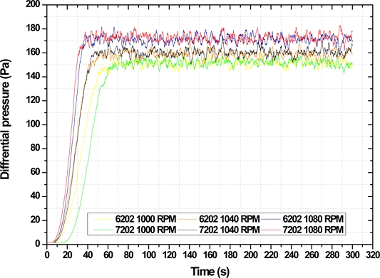
In this study, the bearing defects were ball-wear defects and contamination. Fig. 5 compares the internal differential pressure of the fan-filter unit for the ball bearing at different motor speeds. Similar internal differential pressures were observed for the different bearings at motor speeds of 1,000, 1,040, and 1,080 RPM.
3.2 Differential Pressure by Defects
The types of defects in the fan filter unit were classified into bearings, filters, and motor defects. Section 3 compared the raw data of the differential pressure for each defect’s state to visualize and determine the difference in differential pressure for each defect.
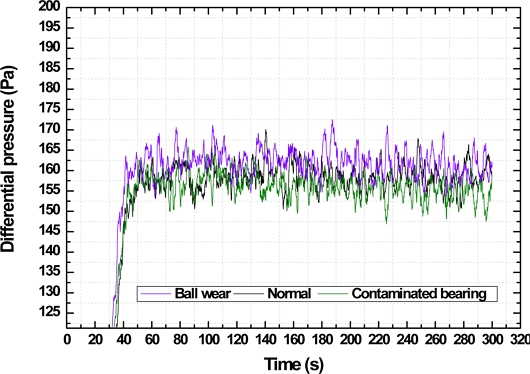
This study classified the bearing defects of the fan filter unit into ball wear defects and internal contamination. The differential pressure inside the fan filter unit was compared with normal bearings, ball wear defect bearings and contamination bearings at a reference motor speed of 1,040 RPM. The average differential pressure for the ball-wear, normal, and contaminated bearings was 162.24, 159.13, and 156.2 Pa, respectively. As shown in Fig. 6, it is confirmed that the differential pressure signal caused by the bearing defect is less different from the normal bearing, despite the large defect that grinder grinds two out of ten balls and pollutes the inside.
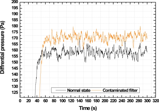
The internal differential pressure was measured for a new and expired HEPA filter. The internal differential pressure of the FFU increases because the pores of the used filter are clogged compared to the normal filter. The average differential pressure for the normal and contaminated filters was 159.13 Pa and 171.01 Pa, respectively. The differences was 11.88 Pa (7.46%), and the results are shown in Fig. 7.
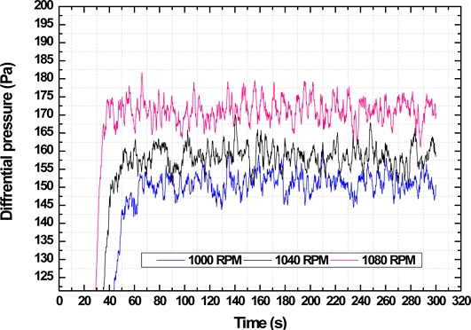
The internal differential pressure of the fan-filter unit at 1,000 and 1,080 RPM was measured using a speed regulator at a reference speed of 1,040 RPM. The average value of the differential pressures was 171.57 Pa, 159.13 Pa, and 150.71 Pa for 1,080, 1,040, and 1,000 RPM, respectively. The differences between the average differential pressures from the reference speed of 1,040 RPM were 12.84 Pa and 8.42 Pa (8.06% and 5.29%) for 1,080 and 1,000 RPM, respectively. The results are shown in Fig. 8.
3.3 Deep Learning
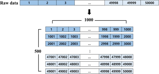
In this study, there is a limit to judging the differential pressure data obtained by each defect only by data. Thus, we used a deep learning diagnostic technique to diagnose defects in the fan-filter unit. We used raw data obtained from differential pressure sensors, reconstructing 500,000 data for each defect into 500*1,000 form, and using it for deep learning experiments. Fig. 9 is shape of data by label.
The deep learning algorithms typically used to detect and diagnose defects in a system are artificial neural network (ANN), deep neural network (DNN), convolutional neural network (CNN), and recurrent neural network (RNN). ANN algorithms are early deep learning algorithms that mimic human neural network principles and structures [19,20]. In ANN algorithms, structures with two or more hidden layers are referred to as DNN algorithms [21]. CNN, an algorithm derived from DNN, extracts data features to identify patterns of features and uses compression and computation processes to classify primarily image-based data [22]. RNN, an algorithm derived from DNN, has a recurrent structure. It uses a circular structure to convey previous data values and is a practical algorithm for continuous and repetitive signal data [23]. Because the defect signal was continuously detected once it occurred, RNN algorithm was determined to be suitable for this experiment.
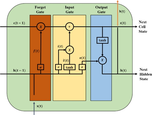
Recurrent neural network algorithms have an Exploding Gradient or Vanishing Gradient problem where the next sequential gradient increases or disappears rapidly as the data get longer [24]. The algorithm that complements this is short- and long-term memory (LSTM) algorithm, as shown in Fig. 10. LSTM algorithms is that solve the problem of RNN algorithm that cause long data by passing only the necessary information to the next time at the current time and deleting unnecessary information [25].
At time step t, the LSTM cell has an input vector [ht-1, xt]. The new cell state, Ct, and the new output, ht, is made by information from previous states, Ct-1 and ht-1 and they send information to the next cell at time step t+1. The output, ht, is determined by the current input, xt, and the previous output, ht-1. LSTM has three gates; forget gate (f), input gate (i) and output gate (o). The forget gate determines which information is discarded or taken from the cell state through the sigmoid layer, an S-shaped curve between zero and one.
Mathematically, the output ft of forget gate is given by Eq. (3). The σ is the sigmoid activation function, Wf is the weight and bf is bias of the forget gate.
| (3) |
The input gate determines which new incoming information is stored in the cell state. First, determine which values to update through the sigmoid layer, and then create a new candidate vector in tanh layer. The tanh layer, the hyperbolic tangent, is similar shape to sigmoid layer, and is between minus one and one. The output it of input gate is given by Eq. (4). Wi is the weight and bi is bias of the input gate. The sigmoid function output in input gate is used to determine which information to update. In contrast, the tanh function is used to determine what new information to add to the cell state, . It is given by Eq. (5).
| (4) |
| (5) |
If the information to be discarded from the previous gate and the information to be updated are determined, update it during the cell state update process. The cell state update is given by Eq. (6). The cell state update is determined by the output of input gate and the output of output gate.
| (6) |
The output gate determines which information to the output. First, input data is put in the sigmoid layer to determine the output information, then cell state is put in the tanh layer, multiplied by the output of the sigmoid layer set it as the output. The output it of input gate is given by Eq. (7). Wo is the weight and bo is bias of the output gate. The output of LSTM, ht, is given by Eq. (8). The ht is transferred to the next step to repeat the above process. Fig. 11 is schematic diagram of LSTM cell structure.
| (7) |
| (8) |
In this study, the defect classification performance of the LSTM model was confirmed when differential pressure data of random defects were set as input data after learning differential pressure data by defect in the LSTM model.
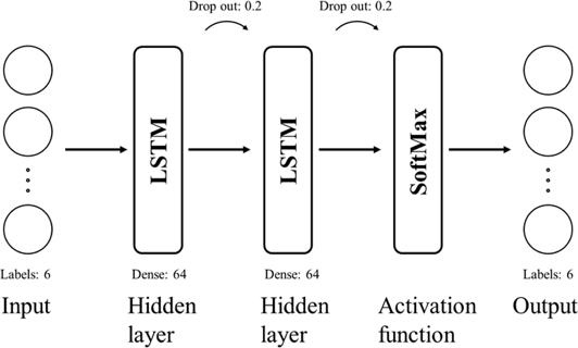
Data labeling is the first step in deep learning model building. As such, labels were assigned to the 1,000 RPM, normal state, 1,080 RPM, internal contaminated bearing, ball-wear bearing, and contaminated filter data. For each label, 500 data and thereby, a total of 3,000 data were obtained. Training, verification, and test data were divided into 1,920, 480, and 600 data at a ratio of 64 : 16 : 20, respectively. The epoch number, batch size, hidden layers, and dropout of the deep learning model were kept at the default setting of 200, 64, 2, and 0.2, respectively. Fig. 12 is schematic of deep learning model. We used GPU-based Tensorflow toolbox, GPU-NVDIA GeForce RTX2060 SUPER, CPU-Intel(R) i5-8500, 16GB memory for deep learning.
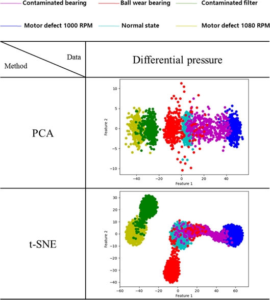
Before conducting the deep learning experiment, clustering between the data was confirmed using principal component analysis (PCA) and t-SNE algorithms, which are low-dimensional mapping techniques. PCA and t-SNE algorithms are a dimensionality-reduction method that is often used to reduce the dimensionality of large data sets, by transforming a large set of variables into a smaller one [26] that still contains most of the information in the large set. The PCA algorithm is an algorithm that projects data between coordinates in one dimension and creates a straight line in the area with the widest data distribution, reducing data loss and clustering [27]. The t-SNE algorithm is a clustering algorithm that finds orthogonal reference points that preserve the variance to the maximum and lists them according to the criteria [28]. Through these algorithm, clustering between data can be visualized and confirmed when dimension is reduced. Fig. 13 is differential pressure data mapping result using dimension reduction method.
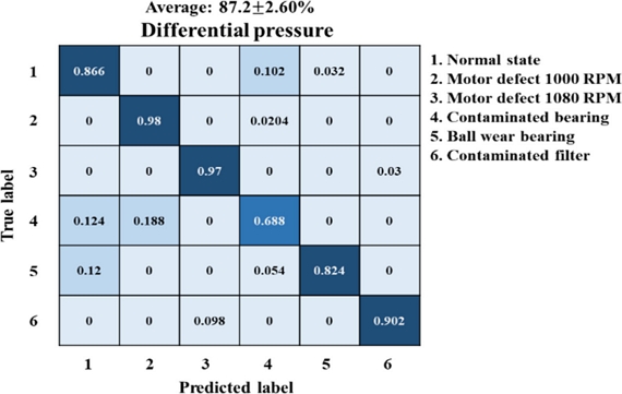
As result of the low-dimensional mapping, it can be seen that the motor defect 1,080 RPM and the filter defect do not fully cluster and overlap to some extent. Similarly, internal contamination bearings, ball defect bearings, and steady state were not fully clustered. Likewise, internal bearings and motor defects 1,000 RPM were not fully clustered. The similar result can be seen in the confusion matrix. The results of the deep learning experiment were randomly mixed and tested five times to evaluate reliability. The defects were classified with an average accuracy of 87.2±2.60%. The deep learning results are presented using confusion matrix, which is a specific table layout that allows easy visualization of the performance of deep learning [28]. Fig. 14 shows the confusion matrix generated by the deep learning experiment.
4. Conclusion
This study proposed a defect diagnosis system for the fan-filter unit of a clean room. Defects in the fan-filter unit were divided into bearing, filter, and motor defects and the internal fan-filter pressure was measured for each defect. Bearing defects included ball wear and contamination; filters were also contaminated, and motor defects were simulated by changing the motor speed.
The acquired data were used to train a deep learning algorithm to diagnose fan-filter unit defects because the measured data alone were limited in diagnosing defects. Six labels were assigned in the order of 1,000 RPM, steady state, 1,080 RPM, internal contaminated bearing, ball-wear bearing, and contaminated filter. Before the deep learning experiment, clustering between data was confirmed using low-dimensional mapping techniques, PCA, and t-SNE algorithms. The confusion matrix evaluated the average value of the randomly mixed data five times to ensure reliability. As a result, defects were classified with an average accuracy of 87.2±2.60%. This confirms the possibility of diagnosing defects in clean-room fan-filter units using only differential pressure sensors.
Acknowledgments
This work was supported by Korea Institute for Advancement of Technology (KIAT) grant funded by the Korea Government (MOTIE) (P0002092, HRD Program for Industrial Innovation) and the National Research Foundation of Korea (NRF) grant funded by the Korea government (MSIT) (NRF-2020R1F1A1072926). We would like to thank Editage (www.editage.co.kr) for English language editing.
REFERENCES
- Jun, C.-S., Kim, H.-J., Park, Y.-M., Lee, D.-W., Ham, D.-S., Jeon, S.-M., Lee, K.-Y., (2007), Wet chemical process for improving air quality in semiconductor manufacturing process, Clean Technology, 13(2), 109-114.
- Holbrook, D., (2009), Controlling contamination: The origins of clean room technology, History and Technology, 25(3), 173-191. https://doi.org/10.1080/07341510903083203
- ISO 14644-6, (2007), Cleanrooms and associated controlled environments Part 6: Vocabulary.
- You, H.-S., Wang, T.-C., Chang, W.-Y., Lai, C.-W., Lee, M.-W., Zuo, K.-w., (2004), Unified framework for facility condition monitoring, detection, and diagnostics, Proceedings of the Semiconductor Manufacturing Technology Workshop Proceedings, 41-46.
-
Zajic, I., Larkowski, T., Hill, D., Burnham, K. J., (2010), Temperature model of clean room manufacturing area for control analysis, Proceedings of the UKACC International Conference on CONTROL, 1251-1256.
[https://doi.org/10.1049/ic.2010.0460]

-
Sunardi, A., Agus, D., Aditya, H., Susila, W., (2019), Online air velocity control, temperature and humidity monitoring system for clean room using Raspberry Pi, Proceedings of the IOP Conference Series: Materials Science and Engineering, 012011.
[https://doi.org/10.1088/1757-899X/550/1/012011]

- Vázquez Amaro, L. J., (2019), Clean room differential pressure monitoring improvements. https://prcrepository.org/handle/20.500.12475/305
-
Savage, G., (2007), Failure prevention in bonded joints on primary load bearing structures, Engineering Failure Analysis, 14(2), 321-348.
[https://doi.org/10.1016/j.engfailanal.2005.11.013]

-
Liang, J., Du, R., (2007), Model-based fault detection and diagnosis of HVAC systems using support vector machine method, International Journal of Refrigeration, 30(6), 1104-1114.
[https://doi.org/10.1016/j.ijrefrig.2006.12.012]

-
Shahnazari, H., Mhaskar, P., House, J. M., Salsbury, T. I., (2019), Modeling and fault diagnosis design for HVAC systems using recurrent neural networks, Computers & Chemical Engineering, 126, 189-203.
[https://doi.org/10.1016/j.compchemeng.2019.04.011]

-
Taheri, S., Ahmadi, A., Mohammadi-Ivatloo, B., Asadi, S., (2021), Fault detection diagnostic for HVAC systems via deep learning algorithms, Energy and Buildings, 250, 111275.
[https://doi.org/10.1016/j.enbuild.2021.111275]

-
Mongia, C., Goyal, D., Sehgal, S., (2022), Vibration response-based condition monitoring and fault diagnosis of rotary machinery, Materials Today: Proceedings, 50, 679-683.
[https://doi.org/10.1016/j.matpr.2021.04.395]

- KS B 6740, (2015), Performance test methods for clean room-air filters.
-
Elnour, M., Meskin, N., (2020), Actuator fault diagnosis in multi-zone HVAC systems using 2D convolutional neural networks, Proceedings of the 2020 IEEE International Conference on Informatics, IoT, and Enabling Technologies (ICIoT), 404-409.
[https://doi.org/10.1109/ICIoT48696.2020.9089508]

-
Reppa, V., Papadopoulos, P., Polycarpou, M. M., Panayiotou, C. G., (2014), A distributed architecture for HVAC sensor fault detection and isolation, IEEE Transactions on Control Systems Technology, 23(4), 1323-1337.
[https://doi.org/10.1109/TCST.2014.2363629]

-
Hong, D., Kim, W., (2014), Quantitative NDE thermography for fault diagnosis of ball bearings with micro-foreign substances, Journal of the Korean Society for Nondestructive Testing, 34(4), 305-310.
[https://doi.org/10.7779/JKSNT.2014.34.4.305]

- Son, D.-H., Kim, B.-K., Hwang, D.-H., Cho, Y.-H., (2008), Detecting the air-gap flux of the stator fault in induction motor, Proceedings of the Korean Institute of Electrical Engineers Conference, 968-969.
-
Kang, Y., Wang, J., Yang, G., Xiong, X., Chen, X., Yu, L., Zhang, P., (2011), Preparation of porous super-hydrophobic and super-oleophilic polyvinyl chloride surface with corrosion resistance property, Applied Surface Science, 258(3), 1008-1013.
[https://doi.org/10.1016/j.apsusc.2011.07.106]

- Yegnanarayana, B., (2009), Artificial neural networks, Eastern Economy Edition. (https://books.google.co.kr/books?hl=ko&lr=&id=RTtvUVU_xL4C&oi=fnd&pg=PR9&dq=Yegnanarayana,+B.,+(2009),+Artificial+neural+networks,+Eastern%0D%0AEconomy+Edition&ots=Gde0xjwJVw&sig=ZjvAc-Tu-YDpOZ9J3gWbsO52MSk#v=onepage&q=Yegnanarayana%2C%20B.%2C%20(2009)%2C%20Artificial%20neural%20networks%2C%20Eastern%20%20Economy%20Edition&f=false)
-
Sathish, T., Karthick, S., (2018), HAIWF-based fault detection and classification for industrial machine condition monitoring, Progress in Industrial Ecology, an International Journal, 12(1-2), 46-58.
[https://doi.org/10.1504/PIE.2018.095870]

- Larochelle, H., Bengio, Y., Louradour, J., Lamblin, P., (2009), Exploring strategies for training deep neural networks, Journal of Machine Learning Research, 10(1), 1-40. https://www.jmlr.org/papers/volume10/larochelle09a/larochelle09a.pdf
-
Yamashita, R., Nishio, M., Do, R. K. G., Togashi, K., (2018), Convolutional neural networks: An overview and application in radiology, Insights into Imaging, 9, 611-629.
[https://doi.org/10.1007/s13244-018-0639-9]

-
Medsker, L., Jain, L. C., (1999), Recurrent neural networks: Design and applications, CRC Press.
[https://doi.org/10.1201/9781420049176]

-
Li, S., Li, W., Cook, C., Zhu, C., Gao, Y., (2018), Independently recurrent neural network (indrnn): Building a longer and deeper rnn, Proceedings of the IEEE Conference on Computer Vision and Pattern Recognition, 5457-5466.
[https://doi.org/10.1109/CVPR.2018.00572]

-
Yu, Y., Si, X., Hu, C., Zhang, J., (2019), A review of recurrent neural networks: LSTM cells and network architectures, Neural Computation, 31(7), 1235-1270.
[https://doi.org/10.1162/neco_a_01199]

- Roweis, S., (1997), EM algorithms for PCA and SPCA, Advances in Neural Information Processing Systems, 10. https://proceedings.neurips.cc/paper_files/paper/1997/hash/d9731321ef4e063ebbee79298fa36f56-Abstract.html
- Van Der Maaten, L., (2014), Accelerating t-SNE using tree-based algorithms, The Journal of Machine Learning Research, 15(1), 3221-3245.
-
Stehman, S. V., (1997), Selecting and interpreting measures of thematic classification accuracy, Remote Sensing of Environment, 62(1), 77-89.
[https://doi.org/10.1016/S0034-4257(97)00083-7]


M.S. degree graduate in the Department of Smart Health Science and Technology, Kangwon National University. His research interest is fault detection and diagnosis.
E-mail: cotur1215@kangwon.ac.kr

Post-Doctorate researcher candidate in the Department of Smart Health Science and Technology, Kangwon National University. His research interest is micro/nanoscale surface texturing technologies and the design of medical devices and AI application system design.
E-mail: wkddndrl@kangwon.ac.kr

M.S. degree graduate in the Department of Mechatronics Engineering, Kangwon National University. and R&D with SPM Instrument Korea. His research interest is fault detection and diagnosis.
E-mail: kjh@spminstrmentkorea.co.kr

M.S. candidate in the Department of Smart Health Science and Technology, Kangwon National University. His research interest is ultrasonic cutting.
E-mail: dhwan465@naver.com

Professor in the Department of Mechatronics Engineering, Kangwon National University. His research interest is Korean bells, sound insulation of the railway vehicle, vibration and noise analysis of the wind turbine, and so on.
E-mail: seock@kangwon.ac.kr
Professor in the Department of Smart Health Science and Technology, Kangwon National University. His research interest is micro/nanoscale surface texturing technologies and their applications in various sensor system.
E-mail: mems@kangwon.ac.kr

Professor in the Department of Smart Health Science and Technology, Kangwon National University. His research interest is micro and nano system design and precision control of machine tools he design of medical devices and AI application system design.
E-mail: kbh@kangwon.ac.kr
