Degradation Pattern Classification for Predicting Remaining Useful Life of Rolling-element Bearings
Copyright © The Korean Society for Precision Engineering
This is an Open-Access article distributed under the terms of the Creative Commons Attribution Non-Commercial License (http://creativecommons.org/licenses/by-nc/3.0) which permits unrestricted non-commercial use, distribution, and reproduction in any medium, provided the original work is properly cited.
Abstract
In continuous-process systems, failures of rolling-element bearings typically cause accidents, reduced productivity, and production-related financial losses. Therefore, predicting both the lifespan of rolling-element bearings and their replacement time is crucial for preventing machine system failures. Accordingly, numerous studies have reported various machine and deep learning classifiers for predicting the lifespan of bearings. However, these studies did not consider degradation trends of bearings. Thus, this study aimed to develop an algorithm to predict the lifespan of a bearing by considering its degradation trend. A vibration dataset of bearings was obtained at low and high speeds. Using a second-order curve-fitting model, various degradation patterns in the dataset were classified. Appropriate time-domain or frequency-domain feature variables applicable to the design of a classifier were determined according to classified patterns. In addition, the classifier was trained using multiple bidirectional long short-term memories. Finally, the performance of the developed classifier was verified experimentally
Keywords:
Degradation, Feature engineering, Remaining useful life, Rolling-element bearings, Prediction키워드:
열화, 특징공학, 잔여수명, 구름 베어링, 예측1. Introduction
Unexpected failure of rolling-element bearings in a machine system typically causes several problems. In continuous-process systems such as roll-to-roll systems, where productivity is critical, defects in rolling-element bearings result in equipment failures, poor product quality, production delays, and financial losses [1]. High-speed rotating equipment, like turbines and railways, face serious accident risks due to bearing failures [2,3]. According to Buchaiah and Shakya [4], bearing-related failures account for more than 40% of all industrial motor failures. Therefore, predicting the accurate and reliable remaining useful life (RUL) of bearings is crucial for preventing and repairing mechanical system failures [3-7].
RUL prediction methods include model-based and data-based approaches [3]. Model-based methods use mathematical models of physical phenomena to predict the RUL of bearings. This method includes the autoregressive integrated moving-average approach [8], Paris crack growth model generation method (in which the growth of cracks in the bearing is considered physically [9]), Kalman filters [10], and particle filters [11]. However, the modelbased residual-life prediction method is limited in its application to various systems, including bearings, because it requires the development of a mathematical model for each system. In addition, the more complex the system, the longer it takes to create a mathematical model and the greater the number of equation variables required for lifespan determination. Consequently, the amount of system-related information that needs to be known increases. Therefore, recent research in this field has focused on data rather than on model-based methods [12].
Data-driven RUL prediction acquires bearing condition information from previously obtained data [3]. Two types of datadriven methods have been proposed: artificial intelligence (AI) and statistical methods. Among the actively studied AI methods, this study introduced RUL-prediction methods using deep learning. The deep-learning-based RUL-prediction method automatically secures the RUL-related pattern from obtained data, and its generalization is superior to that of the statistical RUL-prediction method, which sets an artificial threshold [2].
Predicting the RUL based on deep learning involves six steps [4]. The first step is data acquisition, wherein the vibration data of the bearing are recorded using an acceleration sensor to obtain raw data. The second step is feature extraction, in which the amount of data is reduced and numerical indicators showing bearing conditions are extracted. Oh et al. [13] diagnosed rotary machine conditions using 12 characteristic variables, including the mean, root mean square (RMS), skewness, and kurtosis. The third step is feature selection, which extracts a feature variable that can increase the prediction accuracy of the RUL model among several feature variables. Lei et al. [3] introduced monotonicity, robustness, trendability, and consistency as RUL-prediction accuracy indicators. The predictive model was trained using the highest feature index or an index that exceeded a predefined threshold. Lee et al. [14] proposed a method for selecting raw data based on the directional nature of faults and for selecting a feature variable based on a feature combination matrix for the fault diagnosis of mechanical systems. The fourth step is data fusion, in which only the RULrelated features are extracted by reducing the dimensions of the selected feature variables for a more accurate prediction. Motahari- Nezhad and Jafari [15] extracted features that increased the accuracy of the state classification of bearings by reducing dimensionality with several feature variables through improved distance evaluation. The fifth step was data preprocessing for highaccuracy fault diagnosis and predictive model generation, and the sixth step was fault diagnosis. Lee et al. [16] classified the state of a rotary machine, including bearings, into four types using empirical mode decomposition and a support vector machine. Chen et al. [17] determined the presence and type of bearing defects in the frequency band based on a resonance-based sparse signal (RSSD) and wavelet transform.
The last step is RUL prediction, in which the RUL is determined by generating a predictive model based on the defect information obtained in the previous step. Ali et al. [18] reduced the fluctuations included in the existing time-domain feature variables with the universal failure rate function and learned the RULprediction model of the bearing based on an artificial neural network. Ren et al. [19] predicted the RUL of multi-bearings using frequency spectrum partition summation, extracted based on a deep neural network and Fourier transformation. Alguacil et al. [20] estimated the propagation of acoustic waves based on deep convolutional neural networks (DCNN). Zhu et al. [21] proposed a method to predict the RUL by training a multiscale convolution neural network with time-frequency representations. Li et al. [22] developed a multiscale DCNN (MS-DCNN) to extract only features suitable for RUL prediction from complex and diverse feature variables. Therefore, numerous prediction models based on deep learning have been proposed. However, neural networks do not consider the sequence between time-series learning data; hence, they only learn the data at a certain point. In addition, as the amount of data increases, long-term dependency occurs. Consequently, a model that reflects only the features of the learned data was constructed [23]. Therefore, the prediction error of RUL is calculated by considering the characteristics of each dataset, and the sequential change pattern may increase.
Numerous studies on recurrent NNs (RNNs) [24] have been conducted to obtain a model with higher prediction accuracy by learning sequentially ordered time-series data. Guo et al. [25] used an RNN health indicator (HI) as a HI based on an RNN, thereby reporting the condition of bearings. Experimentally, they demonstrated that the RNN-HI exhibited higher monotonicity and correlation values in relation to the RUL-prediction accuracy compared with that of the HI generated from existing feature variables. Hinchi et al. [26] extracted the local features using a convolutional layer. They predicted the RUL of a bearing through a long short-term memory (LSTM) layer designed to solve the long-term dependency problem, which has not been solved in traditional RNNs. Luo et al. [27] integrated multi-Gaussian fitting and LSTM (GaPSD/LTSM) for accurate structural health prediction. Zhang et al. [28] evaluated the performance degradation of bearings using LSTM RNNs, and predicted the RUL based on this. Chen et al. [29] accurately predicted the RUL by applying the attention mechanism to the existing LSTM and frequency band derived from the fast Fourier transform (FFT). Haidong et al. [30] proposed a method for the early detection of bearing failure using a gated recurrent unit with a simpler calculation method than the LSTM and complex wavelet packet energy moment entropy. Cheng et al. [31] predicted the degradation indicator and RUL of bearings using an RNN with a bidirectional LSTM (bi-LSTM) structure. Existing studies in this field have predicted the RUL of all bearings by developing a single RUL-prediction model. However, different vibration patterns can be obtained owing to the manufacturing process, the condition of the equipment connected to the bearing, and lubrication condition, even if the actual bearing is analyzed under identical conditions [32]. Therefore, for accurate RUL prediction, the degradation pattern of the bearing must be classified beforehand.
We developed an RUL-prediction algorithm that includes a degradation pattern classification step after data fusion and feature selection. The degradation pattern classification process was performed based on quadratic curve fitting, and a decision on the use of time-domain or time-frequency domain features was made based on the classification results. Curve fitting was applied to one feature selected based on the Laplacian score (LS) among several time-domain features [33]. If RUL prediction was deemed possible based on time-domain features, the LS feature was used for RUL prediction.
Conversely, if RUL prediction was deemed possible using timefrequency domain features, it was predicted using the decreasing frequency bands proposed in this study. Here, the decreasing frequency bands refer to the bands with the smallest values obtained by applying Pearson's linear correlation coefficient to the frequency bands. The size of the proposed feature decreases as the defect becomes more severe, and it has the characteristic of a defect signal that is difficult to identify from the time-domain features. Therefore, even when time-domain features that remain unchanged with time—owing to weak defects—are extracted, degradation patterns capable of checking the decreasing frequency bands can be secured, and the RUL-prediction accuracy can be improved. Prior to the learning stage of the RUL-prediction model, the point at which RUL prediction was possible was identified by classifying the bearing state using moving-average filtering and k-means clustering. As a feature of a predictable time period, an RULprediction model was trained using an RNN with multiple bi-LSTM structures. The RUL predicted by the proposed method was found to have higher accuracy than that predicted by another method.
The remainder of this paper is organized as follows. Section 2 explains the theories used in the proposed RUL-prediction algorithm. Section 3 introduces the proposed RUL-prediction algorithm. Section 4 describes the experiment conducted to verify the accuracy of the proposed RUL-prediction algorithm. Section 5 presents the results obtained when the prediction algorithm was applied to the data obtained experimentally. Finally, Section 6 summarizes the conclusions of the study based on an analysis of the results and future research directions.
2. Theories for the Proposed Remaining Useful Life (RUL) Prediction Algorithm
The proposed algorithm is derived from four existing theories, namely, feature extraction, LS, Pearson's linear correlation coefficient, and bi-LSTM, introduced in this section. First, in feature extraction, time-domain, and time-frequency domain features are introduced as statistical indicators. The LS and Pearson's linear correlation coefficient are indicators for selecting one of several characteristic variables, and each subsection explains the underlying concept. Finally, bi-LSTM was used as a neural network structure for learning RUL models. In this section, bi-LSTM and the concepts of RNN and LSTM are discussed.
2.1 Time-domain Feature Extraction for Defect Magnitude Identification
In this study, time-domain features were extracted using 14 statistical indicators. Table 1 lists the names, equations, descriptions, and uses of the 14 time-domain features. The method and meaning of bearings are different for each characteristic variable. For example, RMS represents the average magnitude of the vibration of a bearing, whereas skewness represents the imbalance of the bearing [16].
The mean calculates the average value of the vibration signal, providing a basic measure of central tendency. Its strength lies in its simplicity and ease of interpretation, which helps establish a baseline for signal analysis. However, because the mean is sensitive to noise and outliers, it may not effectively capture the dynamic changes crucial for diagnosing bearing health. In this study, while the mean offers initial insights, its limitations necessitate deeper analysis with more robust features for accurate RUL predictions.
The absolute mean highlights the average magnitude of vibration signals regardless of directionality. Its robustness against negative values is a strength when dealing with bipolar signal oscillations. However, like the mean, it lacks sensitivity to detailed signal changes that are essential for predictive accuracy in RUL modeling. In this study, the absolute mean provided foundational data, but its standalone predictive power was limited.
This feature extends RMS analysis by focusing on the squared amplitudes, which enhances sensitivity to significant signal deviations. Its strength is in highlighting subtle shifts in vibration severity. Yet, its complexity can mask minor faults unless paired with other discriminating features. This study incorporated amplitude of RMS to refine the detection of degradation stages, aligning closely with RUL estimates.
As a measure of the full oscillation range, peak to peak provides a snapshot of signal extremity that can indicate severe bearing issues. Its direct approach simplifies identification of significant anomalies. Nonetheless, it may overlook gradual degradation not reflected in extreme values. This research found peak to peak useful in detecting abrupt failures, yet it worked best when integrated with comprehensive trend analysis.
Standard deviation quantifies signal dispersion around the mean, offering insights into variability. Its strength is in capturing the consistency of operation, where deviations might signal upcoming faults. However, excessive focus on variability can miss the larger degradation arc. This study leveraged standard deviation to flag inconsistent vibration patterns, facilitating early-stage warning detection.
Kurtosis measures signal impulsiveness, effectively identifying sudden impacts or shocks. Its role in highlighting extreme deviations supports detection of abrupt defects. However, sensitivity to noise requires careful application. In the findings, kurtosis helped reveal infrequent, high-impact events that could undermine RUL reliability if unchecked.
The form factor relates waveform shape consistency by comparing RMS to absolute mean, aiding in identifying vibration uniformity. Its strength lies in its ability to detect changes in waveform dynamics. However, it can miss small-scale deviations crucial for predicting gradual RUL changes. The study employed form to validate uniform machine operation and detect waveform consistency issues.
Peak value reflects the maximum signal magnitude, directly indicating potential extreme force events or imminent failures. While straightforward, its focus on top values might not represent consistent degradation patterns. This study utilized peak values to accentuate potential high-risk periods, albeit complemented by continuous trend monitoring.
Margin expresses the ratio of peak to RMS amplitude, highlighting transient spikes. It aids in identifying sudden stress points in vibration data. However, its narrow focus requires additional features for contextual completeness. Throughout this study, margin was pivotal for isolating spikes often precursors to significant RUL decline.
Pulse, or peak to absolute mean ratio, underscores sporadic intensity shifts. It is potent in recognizing momentary heightened activity within bearings. Though indicative of acute issues, it lacks comprehensive fault context. This study leveraged pulse measurements to encapsulate fluctuating stress indicators, tying them with broader signals to approximate degradation.
Crest factor, the peak to RMS ratio, is adept at identifying signal outliers and abnormal peaks, providing a quick health status check. However, its oversensitivity to isolated peaks can detach it from meaningful trends. Within our results, crest factor served as a rapid first-level check for anomalies before deeper analysis. Energy represents cumulative signal power, serving as a comprehensive defect indicator over time. Its strength is capturing long-term vibration exposure, an essential
Equal consideration was given to the amount of data obtained for a feature variable and the sampling frequency applied for the data acquisition. Therefore, the number of statistical index values obtained was equal to the actual measurement duration.
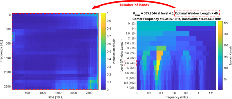
The time-domain features are derived from the size distribution of raw data, whereas the time-frequency domain features used in this study are feature variables that consider both the time and frequency aspects of the bearing size and frequency bands. To obtain the frequency bands, frequency analysis was performed at regular time intervals using FFT, followed by averaging the amplitudes of the signals within a constant frequency band. Fig. 1 shows an example of a frequency band obtained using spectral kurtosis [34]. Particularly, spectral kurtosis is an indicator of impulsiveness according to the frequency band of the signal. The entire frequency band of the signal was decomposed by the window length, which indicated the number of signals to be decomposed, and kurtosis was calculated. Subsequently, the window length with the highest spectral kurtosis was determined to be the optimal length, which was used as the number of frequency bands. The highest spectral kurtosis indicates that the defect signal can be clearly identified if the entire frequency band of the raw signals is decomposed using the corresponding window length. Therefore, the defect signal should be secured using spectral kurtosis to accurately calculate the predicted RUL based on timevarying signal pattern analysis.
2.2 Laplacian Score (LS) for Time-domain Feature Selection
LS is an index used to select feature variables and is a method for unsupervised data classification learning [35]. The characteristics of LS allow for the best preservation of the local characteristics inherent in the data, thereby preserving the distinctive characteristics of the measured data at each time within the time-series data [36]. The variable that most accurately predicts the RUL is the variable size under different bearing conditions. The characteristic variable for learning the RUL-prediction model through LS was selected because it improves classification quality [33]. LS is a function of similarity Sij and variance Var(fn), as shown in Eqs. (1) and (2).
| (1) |
| (2) |
where fn is the nth feature variable among several feature variables and is expressed as fn = [fn1, fn2, ..., fnm]; Sij indicates the similarity between the relationship between each data point and the neighborhood of the data; t is a fixed value that defines the sensitivity to the difference between the two data points, fni and fnj; and Var(fn) is the variance between the elements constituting feature variable fn. To minimize LSn, Σij(fni − fnj)2Sij must be minimized. Therefore, a feature variable that can minimize (fni − fnj) must be selected.to select an LS-based ideal feature variable.
2.3 Pearson’s Linear Correlation Coefficient for Variable Relationship Determination
Pearson’s linear correlation coefficient was used to analyze the proportional and inverse relationships between the two variables, as shown in Eq. (3).
| (3) |
In Eq. (3), the correlation coefficient is calculated from [-1, 1]. Depending on its value, the relationship between the two variables can be defined differently. When the correlation coefficient becomes zero, the two variables become independent. When the value is negative, the two variables are inversely proportional. If the coefficient is -1, the two variables can be defined as linearly decreasing functions. If the coefficient is positive, it exhibits a proportional relationship. If it is +1, the two variables can be defined as linearly increasing functions.
Pearson’s linear correlation coefficient is a statistical measure that evaluates the strength and direction of a linear relationship between two variables. The coefficient, denoted as (r), can take a value between -1 and 1. Each of these values has a specific interpretation that helps in understanding the correlation between variables. A correlation of 1 indicates a perfect positive linear relationship. When (r = 1), one variable increases in direct proportion to the other. In the context of our study, this might reflect how an increasing vibration amplitude directly correlates with a decreasing RUL, demonstrating predictable degradation over time. Conversely, a correlation of -1 represents a perfect negative linear relationship, where an increase in one variable corresponds with an equivalent decrease in the other. This could be observed when increases in defect severity are linked to reductions in structural integrity indicators within the bearing data. An (r) value of 0 signals no linear correlation between the variables. In this case, fluctuations in one variable are independent of changes in the other. This lack of correlation may appear when investigating aspects not directly affected by linear degradation paths, suggesting the influence of non-linear or complex relationships.
Beyond these extreme values, practical applications of Pearson’s correlation involve assessing varying degrees of relationship strength. For the strong positive correlation (0.7 to 0.9) this range suggests a significant positive relationship, where one variable tends to increase as the other does. For instance, this relationship might be evident between cumulative operational load and progressive wear indicators, where consistently increasing stress results in heightened wear.
A moderate positive correlation (0.3 to 0.7), indicates a noticeable, though not definitive, positive relationship. For example, increased vibration frequency might correlate moderately with temperature rise, hinting at a possible effect of heat on bearing wear, albeit with influencing factors.
For a weak positive correlation (0 to 0.3), a slightly positive trend may be observed, reflecting marginal links between variables such as minor lubrication fluctuations affecting vibration signals. These weak correlations suggest potential causal factors requiring further investigation. Similarly, negative correlations across these scales reflect inversely proportional relationships, often crucial in understanding diminishing trends between operational variables and failure statistics. Incorporating detailed interpretations of Pearson’s correlation allows for nuanced insights into the variable interactions observed in bearing performance data, thus enhancing the robustness of predictive modeling in this study. This expanded perspective on Pearson’s linear correlation facilitates a comprehensive examination of relationships within the dataset, ensuring a more thorough analysis and interpretation of bearing degradation patterns.
2.4 Bidirectional Long Short-term Memory (bi-LSTM) Suitable for Time-series Data Training
An RNN is a model that processes input and output data in sequence units and is trained using a supervised learning method. Here, the input data were the feature variables selected based on the LS, and the output data were defined as the RUL of the timeseries data. We assumed that the amount of RUL data decreased linearly with time because they could not be obtained directly by measuring equipment, such as sensors.
A typical RNN comprises input, hidden, and output layers. The hidden layer obtained in the previous period has a structure that affects the computation of the hidden layer in the subsequent period. The hidden layer stores the characteristics of the data obtained from the input layer, and is composed of weights, biases, and activation functions.
However, a simple RNN structure is limited by its long-term dependence. During model training, the previously learned data characteristics are lost owing to long-term dependence, and the model learns only the input data characteristics entered later. To address this problem, an LSTM structure was proposed. An LSTM learns the model by classifying the hidden layer into short- and long-term states, and gate controllers, including forget, input, and output gates, are added to the structure of the existing RNN. The activation function σ for calculating each gate value employs a function whose output value is defined as [0, 1], such as sigmoid and logistic functions. If the output value is 1, then the input and hidden state values of time are passed. This LSTM structure learns time-series data in one direction.
Bi-LSTM improves learning performance by considering both directions of time. It is advantageous for learning data patterns because it considers the direction of data and allows for the balanced learning of all data over the entire time period. When learning the data using this structure, each gate is calculated as a vector, and the state value ht of the hidden layer is obtained using Eq. (4).
| (4) |
where ht is the state value of the calculated hidden layer, and () and () denote those of the hidden layer calculated in the forward and backward directions, respectively. The process for obtaining the state value of the hidden layer for each direction was the same as that used in the existing LSTM structure.
3. Methodology
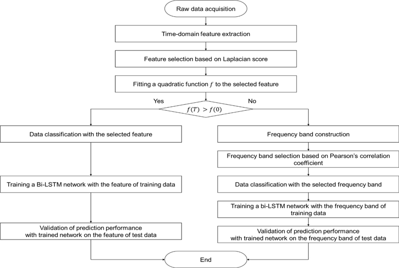
The proposed algorithm for the RUL prediction of bearings with different deterioration patterns is shown in Fig. 2. The primary distinction between the proposed and existing algorithms lies in the use of different feature variables based on the quadratic function fitting results. The feature variable selected for each data point considers deterioration patterns, which can provide information regarding the RUL [37]. Consequently, the proposed algorithm can extract feature variables associated with deterioration patterns, and training the RUL-prediction model with feature variables can improve prediction accuracy.
3.1 Quadratic Function Curve Fitting for Degradation Pattern Classification
The vibration data from the bearings were transformed into 14 time-domain features. Using the LS, a suitable feature for RUL prediction was selected from the transformed features. Subsequently, the values at the beginning and end of the data measurement were compared by fitting the selected features to a quadratic function. If the final value was greater than the initial value, it was used to train the RUL-prediction model and calculate the prediction value using the selected time-domain feature. Conversely, if it was greater at the beginning of the measurement, the RUL predictive model was trained, and the predicted value was calculated using the time-frequency features. This criterion was Fig. 2 Proposed RUL prediction algorithm for rolling-element bearings established because the time-domain features are values generated based on the size and size distribution of the raw data; as the size increases, the defects affecting the RUL become more severe. In addition, the reason for fitting polynomials is that, when comparing values through features, obtaining accurate values is challenging owing to noise and fluctuation. Therefore, RUL prediction was performed based on the pattern of features throughout the entire period.
3.2 Decreasing Frequency Band based on Pearson’s Linear Correlation Coefficient
If the quadratic function fitting determined that the data were unpredictable with time-domain features, the RUL was predicted using the frequency bands. We developed an RUL-prediction algorithm that includes a degradation pattern classification step after data fusion and feature selection. A method for using all the bands used to learn the RUL-prediction model and validate the prediction performance, as well as for selecting only one or several bands from among the available bands, has been proposed. However, when all frequency bands were learned, the RULprediction performance was comparable to that of training on existing raw data. This indicates that the method is inappropriate for data that are determined to be unpredictable with time-domain features based on a quadratic function. Therefore, one RULprediction band was selected using Pearson's linear correlation coefficient.
The selection criterion for a band among several bands is set as the change in the vibration amplitude of the band that most closely resembles the first-order decreasing function as time progresses. Such a physical selection criterion is based on the fact that when a defect occurs, the frequency band with the largest magnitude changes, and a frequency band with a relatively smaller magnitude occurs. This phenomenon is known as an energy shift in the frequency band [38]. By decreasing the frequency band, which decreases in size over time, the characteristics of signals that are difficult to confirm based on raw data can be extracted. The smallest band was defined as a decreasing frequency band by calculating Pearson's linear correlation coefficient of each frequency band with time. This is because the closer the Pearson’s linear correlation coefficient is to -1, which is the smallest value, the greater the change in the band size with respect to time in the form of a linearly decreasing function.
3.3 Classification of Bearing State
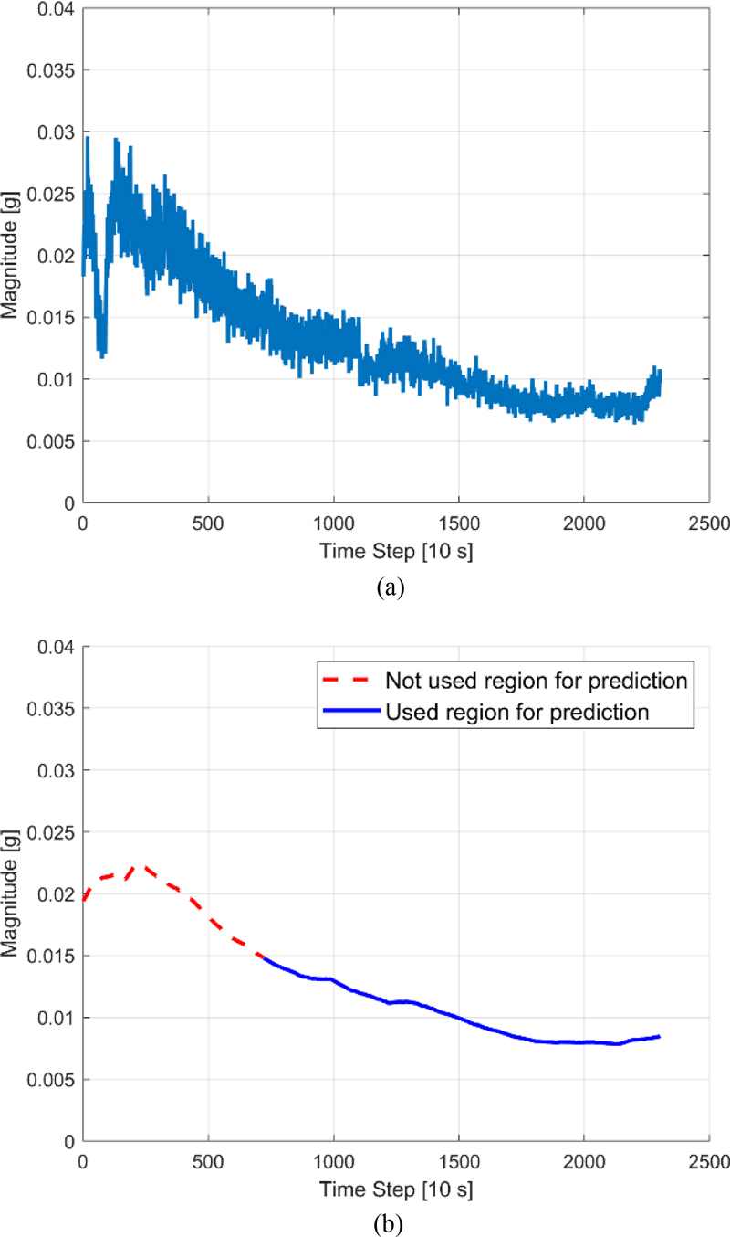
Fig. 3 (a) depicts a decreasing frequency band generated based on the vibration data of the bearing. If a feature is selected based on Pearson's linear correlation coefficient, the data can be confirmed to change rapidly at a specific point, rather than exhibiting a constant decrease. This is because the minimum value of the coefficient for the frequency bands was not completely -1. The vibration magnitude in each frequency band of the bearing changes rapidly owing to the impact when the bearing is physically defective. When training an RUL-prediction model, rapidly changing features can reduce prediction accuracy. In addition, accurate residual-life prediction results can only be obtained when all bearings are in identical conditions at the beginning of the RUL prediction. Therefore, to obtain a model with a high RULprediction accuracy, the state classification of the features should be performed prior to model training.
Therefore, in this study, state classification was performed using moving-average filtering and k-means clustering. The former method calculates the average by moving a window containing a certain amount of data based on the data measurement time. This reduces the influence of outliers and noise. In contrast, the latter is an unsupervised learning method that has the advantage of defining labels by classifying data through clusters in the absence of output data for the input data. However, the disadvantage of kmeans clustering is that it cannot distinguish outliers. Applying kmeans clustering to the filtered data enables accurate state classification after calculating and replacing data outliers with the average of the surrounding data using moving-average filtering, as shown in Fig. 3(b).
3.4 Multiple bi-LSTM for Generating Models
In this study, a residual-life prediction model was developed using an RNN with the deep multiple bi-LSTM structure employed by Cheng et al. [31]. The multiple bi-LSTM, generated by connecting three bi-LSTM structures, is shown in Fig. 4. By learning the RNN with this structure, a deep learning model with high RUL-prediction accuracy for nonlinear data and data learning with various tendencies can be obtained.
RNNs with multiple bi-LSTM structures are trained using supervised learning. Supervised learning is a method for simultaneously learning input and output data, and the RULprediction model is trained to transform the input data into output data. In this study, the input data included a time-domain feature variable or decreasing frequency band selected by the LS, whereas the output data included a linear RUL ratio. Here, the RUL ratio is defined by Eq. (5).
| (5) |
where t is the time elapsed since the start of the measurement. Therefore, the RUL ratio is defined as the ratio of the remaining RUL to the actual RUL.
4. Experimental Setup
4.1 Run-to-failure Test in Low-speed and High-load Conditions
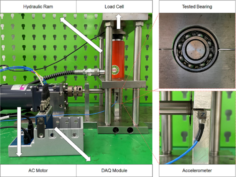
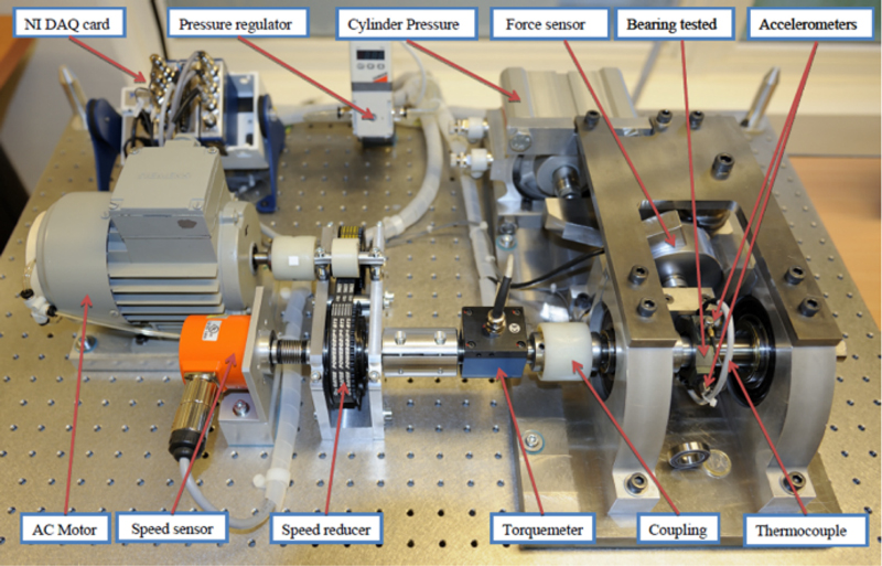
The vibration data must be obtained through a run-to-failure test to evaluate the RUL model of the rolling-element bearings. Fig. 5 shows a bearing test bed used to obtain vibration data, which consists of an AC motor, hydraulic ram, load cell, data acquisition module (DAQ) board and module, accelerometer, and tested bearing. The model of the tested bearing was NSK 6202. First, the bearing vibration measurement process raised the hydraulic ram through a hydraulic pump to apply a desired load to the load cell. Next, while an AC motor was used to rotate the bearing, the vibrations were measured using an accelerometer and DAQ device. The sampling frequency was set to 25,600 Hz when acquiring the data, and the vibration was measured for 1 s every 10 s. Typically, continuous machines, such as roll-to-roll systems, operate at relatively low speeds, unlike rotary machines. Therefore, during the accelerated life test, the vibration was measured at 300 rpm, which is the maximum rotation speed of an AC motor with a 1/6 gear ratio. Fig. 6 shows the raw data for model training obtained from each measurement and the FFT results confirmed at the beginning and end measurement points. The first and second bearing failures occurred at 21,690 s (No. 1) and 22,480 s (No. 2), respectively.
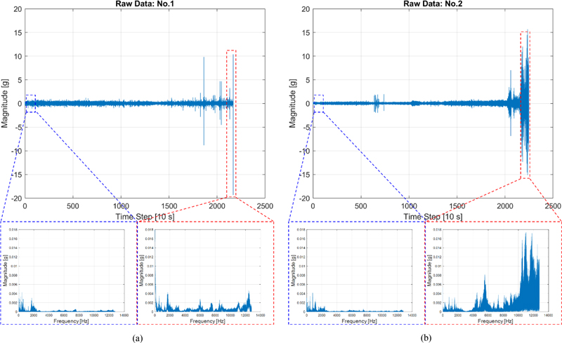
Raw data measured under low-speed conditions and fast Fourier transform (FFT) results: (a) No. 1 and (b) No. 2
Fig. 7 shows the data for evaluating the prediction accuracy of the learned RUL-prediction model; the total measurement time was 22,400 s. However, because RUL must be measured before bearing failure occurs to prevent bearing accidents, data measured at 2,500 s and 5,000 s were removed from the end of the measurement for the same data as in Table 2 and Fig. 7. All measurement data were assigned to No. 3 when RUL = 0, No. 4 when RUL = 2,500 s, and No. 5 when RUL = 5,000 s.
4.2 PRONOSTIA Dataset
To evaluate the RUL of the rolling-element bearings under highspeed and high-load conditions, the PRONOSTIA dataset measured on the same platform, as shown in Fig. 8, was employed. It contains vibration data measured using a run-to-failure test [38] under three acceleration and load conditions, as summarized in Table 3. The vibration signal was obtained for 0.1 s every 10 s, and the sampling frequency was 25,600 Hz.
As presented in Table 4, seven data points measuring bearing vibration in conditions 1 and 2 were provided, whereas only three data points in Condition 3 were provided. Two sets of training data were provided for each condition, and the remaining data were used as test data for the RUL-prediction model. The largest difference between the training and test data was the actual RUL value. If the actual RUL of the training data was zero, the bearing was damaged at the end of the measurement and could no longer be used. Otherwise, the bearing was undamaged even at the end of the data.
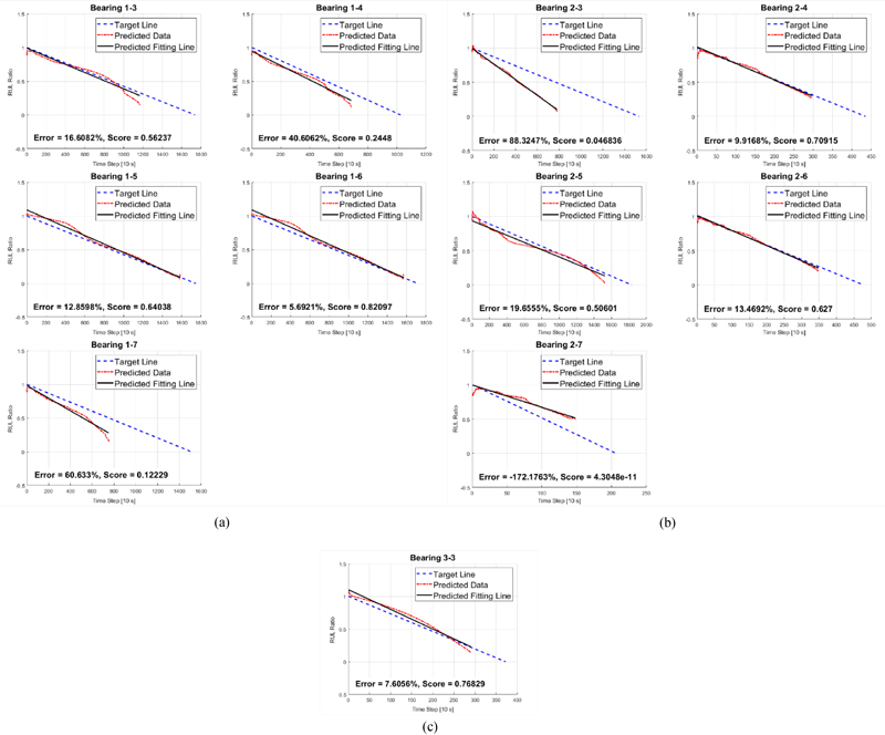
The RUL-prediction result of the verification data is displayed as an error and score and is defined as follows [39]:
| (6) |
| (7) |
Essentially, the closer the error is to 0, the higher the prediction accuracy; the closer the score is to 1, the better the performance of the prediction model. In addition to simple errors, the score is used because a predictive model predicting an RUL that is larger than the actual RUL in a mechanical system is more dangerous than predicting a smaller RUL. If the predicted RUL is larger than the actual value, then the damaged bearing can still be used.
5. Results and Discussion
5.1 RUL-prediction Results for Low-speed Dataset
The proposed algorithm was applied to a vibration dataset obtained under low-speed conditions and used to verify the validity of the algorithm by comparing the actual and predicted RUL. RUL-prediction models were obtained for each feature variable used in deep learning.
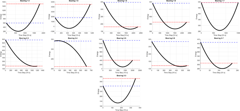
LS is the score obtained for the training dataset, and in this study, energy had the highest score. Therefore, the feature was extracted from the raw data of all test data, and the quadratic function fitting result determined whether to use the energy for the RUL-prediction model or the decreasing frequency band. The defect signal was large at the end of the training data; thus, quadratic function fitting was applied only to the test data, and the results are shown in Fig. 9. The results for No. 5 demonstrated that the defect signal related to the RUL could be effectively extracted using the energy. In addition, extracting the defect signal with energy from the rest of the test dataset was difficult; therefore, the signal had to be classified through frequency analysis.
The number of bands for generating frequency bands, which is a feature variable used for frequency analysis, was determined based on the spectral kurtosis of the training dataset. The spectral kurtosis had the highest value when the number of bands was set to 768, which means that defects were easily found when the frequency was decomposed with the number. The frequency bands generated according to the determined number of bands were obtained using Pearson’s linear correlation. A decreasing frequency band was selected and used to generate an RUL-prediction model for data that could not be predicted with RUL using time-domain features.
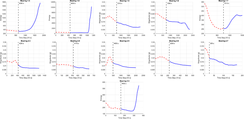
Before training the RUL-prediction model, a decreasing frequency band section was defined using moving-average and kmeans clustering. The starting point of the first prediction interval is defined as the first prediction time (FPT), as shown in Fig. 10. After the prediction interval was defined, each feature variable was converted into cumulative feature variables, which were obtained by accumulating and adding the values of existing feature variables in chronological order. This process was performed to secure an accurate RUL-prediction model by removing noise from existing feature variables.
After learning the RNN with multiple bi-LSTM structures as cumulative feature variables of the training dataset, the RULprediction results of the test dataset were obtained, as listed in Table 5. These results were compared with the energy used in this study and the cumulative feature variables.
The decreasing frequency bands were used individually. The comparison results revealed averages of 778, 4,443, and 1,992 s. when using the proposed algorithm, only energy, and the decreasing frequency band, respectively. Consequently, the prediction error value was reduced when different feature variables were used for RUL prediction, based on the change patterns of the vibration data.
5.2 RUL-prediction Results for PRONOSTIA Dataset
Owing to the frequent use of rolling-element bearings at high and low speeds, the RUL-prediction results were confirmed by applying the proposed algorithm to the PRONOSTIA dataset. The RUL-prediction model was obtained for each condition and each feature variable was utilized for deep learning.
We found that energy received the highest LS score among time-domain features, leading to its selection. The results of quadratic function fitting are shown in Fig. 11. Test data 1-3, 1-4, 1-7, and 3-1 used energy to predict the RUL, whereas the rest of the data predicted the RUL based on decreasing frequency bands. To generate frequency bands, the number of bands for each condition was determined based on the spectral kurtosis of the training data.
As a result of this calculation, 56, 40, and 80 bands were obtained under conditions 1, 2, and 3, respectively. The decreasing frequency band extracted through Pearson’s linear correlation was obtained, and the FPT defined through moving-average and kmeans clustering is shown in Fig. 12. After learning the RNN with multiple bi-LSTM structures as cumulative feature variables of the training data measured in each condition, RUL-prediction results were obtained, as presented in Figs. 13 (a)-(c). Subsequently, these results were compared with those of three study cases in which the prediction results were obtained using the same data [26,28,40], as shown in Table 6. The comparison revealed that when RUL was predicted using the proposed algorithm, the lowest average error was 40.69%, and the highest average score was 0.459.
5.3 Discussion
The results confirmed that the proposed algorithm improved the RUL-prediction accuracy, regardless of the bearing operating conditions. Classifying the characteristic variables used for RUL prediction according to the degradation pattern of bearings based on the comparison results of RUL prediction of bearings operating under low-speed conditions yields more accurate predictions. This implies that, prior to RUL prediction, the bearing degradation pattern must be classified.
In the prediction results for the PRONOSTIA dataset, the absolute error was not the lowest among all validation data. Nevertheless, the average prediction accuracy was high, indicating that the generalization of the prediction model obtained using the proposed algorithm was excellent.
The RUL-prediction results obtained from the two verification datasets confirmed that the prediction accuracy was enhanced when the prediction model was trained with the characteristic variable considering the degradation pattern generated in each dataset. Therefore, for accurate RUL prediction, a suitable characteristic variable for each dataset must be selected by adding a degradation pattern classification process, such as the proposed algorithm. In addition, degradation patterns that are difficult to check in raw data can be extracted through the decreasing frequency band and used for RUL prediction.
6. Conclusion
According to the RUL-prediction results, the degradation pattern was considered a measure for calculating the RUL, and the RUL-prediction model was learned by selecting and considering a characteristic variable. The proposed algorithm was developed by adding a pattern classification step to the existing six steps for predicting the RUL: data acquisition, feature extraction, feature selection, data fusion, fault diagnosis, and RUL prediction. The proposed algorithm requires the generation of multiple predictive models based on the number of classified cases; however, the predictive model can be permanently applied to bearings operating under identical conditions after being generated only once. Moreover, the curve fitting of the predictive model is relatively simpler than that of statistical distributions, such as the beta and Weibull distributions, which is advantageous for real-time RUL predictions.
If time-domain features that are difficult to verify for degradation patterns are extracted based on quadratic function curve fitting, signals with degradation patterns that are difficult to check in existing raw data can be extracted through the decreasing frequency band, and RUL-prediction models can be trained using these. In this case, the prediction accuracy was improved compared to that when only the energy selected through the LS was used. Therefore, even if there is no change in the degradation pattern in the raw data or time-domain features, the degradation pattern must be verified by extracting the decreasing frequency band, because there may be a signal whose size decreases owing to the energy shift caused by degradation.
After classifying the degradation patterns into two, an RULprediction model was developed for each pattern. However, various degradation patterns may appear, depending on the type of bearing, operating conditions, and types of defects. Therefore, if we study how to classify more pattern types by securing additional vibration data for bearings through run-to-failure tests, we can secure models with high RUL-prediction accuracy.
NOMENCLATURE
| σ : | Radial Stress |
| τ : | Stress of Winding Direction |
| b : | Bending Stress |
| ε : | Strain |
| h : | Height |
| m : | Mass |
Acknowledgments
This paper was written as part of Konkuk University’s research support program for its faculty on sabbatical leave in 2024 and the Industrial Fundamental Technology Development Program (No. 20018041, “Development of Energy-saving Low Pressure Injection type Scarfing machine for High-Quality Rolled Steel materials”) funded by the Ministry of Trade, Industry & Energy (MOTIE) of Korea.
References
-
Oh, H., Lee, Y., Lee, J., Joo, C., Lee, C., (2022), Feature selection algorithm based on density and distance for fault diagnosis applied to a roll-to-roll manufacturing system, Journal of Computational Design and Engineering, 9(2), 805-825.
[https://doi.org/10.1093/jcde/qwac028]

-
Liu, R., Yang, B., Zio, E., Chen, X., (2018), Artificial intelligence for fault diagnosis of rotating machinery: A review, Mechanical Systems and Signal Processing, 108, 33-47.
[https://doi.org/10.1016/j.ymssp.2018.02.016]

-
Lei, Y., Li, N., Guo, L., Li, N., Yan, T., Lin, J., (2018), Machinery health prognostics: A systematic review from data acquisition to RUL prediction, Mechanical Systems and Signal Processing, 104, 799-834.
[https://doi.org/10.1016/j.ymssp.2017.11.016]

-
Buchaiah, S., Shakya, P., (2022), Bearing fault diagnosis and prognosis using data fusion based feature extraction and feature selection, Measurement, 188, 110506.
[https://doi.org/10.1016/j.measurement.2021.110506]

-
Liu, H., Mo, Z., Zhang, H., Zeng, X., Wang, J., Miao, Q., (2018), Investigation on rolling bearing remaining useful life prediction: A review, Prognostic System Health Management Conference (PHM-Chongqing), 979-984.
[https://doi.org/10.1109/PHM-Chongqing.2018.00175]

-
Wang, D., Tsui, K.-L., Miao, Q., (2017), Prognostics and health management: A review of vibration based bearing and gear health indicators, IEEE Access, 6, 665-676.
[https://doi.org/10.1109/ACCESS.2017.2774261]

-
Wen, Y., Rahman, M. F., Xu, H., Tseng, T.-L. B., (2022), Recent advances and trends of predictive maintenance from data-driven machine prognostics perspective, Measurement, 187, 110276.
[https://doi.org/10.1016/j.measurement.2021.110276]

-
Kordestani, M., Zanj, A., Orchard, M. E., Saif, M., (2019), A modular fault diagnosis and prognosis method for hydro-control valve system based on redundancy in multisensor data information, IEEE Transactions on Reliability, 68(1), 330-341.
[https://doi.org/10.1109/TR.2018.2864706]

-
Qian, Y., Yan, R., Gao, R. X., (2017), A multi-time scale approach to remaining useful life prediction in rolling bearing, Mechanical Systems and Signal Processing, 83, 549-567.
[https://doi.org/10.1016/j.ymssp.2016.06.031]

-
Singleton, R. K., Strangas, E. G., Aviyente, S., (2015), An improved exponential model for predicting remaining useful life of rolling element bearings, IEEE Transactions on Industrial Electronics, 62(3), 1781-1790.
[https://doi.org/10.1109/TIE.2014.2336616]

-
Qian, Y., Yan, R., (2015), Remaining useful life prediction of rolling bearings using an enhanced particle filter, IEEE Transactions on Instrumentation and Measurement, 64(10), 2696- 2707.
[https://doi.org/10.1109/TIM.2015.2427891]

-
Islam, M. M. M., Prosvirin, A. E., Kim, J.-M., (2021), Datadriven prognostic scheme for rolling-element bearings using a new health index and variants of least-square support vector machines, Mechanical Systems and Signal Processing, 160, 107853.
[https://doi.org/10.1016/j.ymssp.2021.107853]

-
Oh, H., Noh, J., Joo, C., Cho, G., Jo, J., Lee, C., (2023), Classification and redundancy quantitative evaluation algorithm for highly efficient fault diagnosis of rotary machines in roll-toroll systems, Measurement, 206, 112292.
[https://doi.org/10.1016/j.measurement.2022.112292]

-
Lee, Y., Park, B., Jo, M., Lee, J., Lee, C., (2023), A quantitative diagnostic method of feature coordination for machine learning model with massive data from rotary machine, Expert Systems with Applications, 214, 119117.
[https://doi.org/10.1016/j.eswa.2022.119117]

-
Motahari-Nezhad, M., Jafari, S. M., (2021), Bearing remaining useful life prediction under starved lubricating condition using time domain acoustic emission signal processing, Expert Systems with Applications, 168, 114391.
[https://doi.org/10.1016/j.eswa.2020.114391]

-
Lee, J., Park, B., Lee, C., (2020), Fault diagnosis based on the quantification of the fault features in a rotary machine, Applied Soft Computing, 97, 106726.
[https://doi.org/10.1016/j.asoc.2020.106726]

-
Chen, B., Shen, B., Chen, F., Tian, H., Xiao, W., Zhang, F., Zhao, C., (2019), Fault diagnosis method based on integration of RSSD and wavelet transform to rolling bearing, Measurement, 131, 400-411.
[https://doi.org/10.1016/j.measurement.2018.07.043]

-
Ali, J. B., Chebel-Morello, B., Saidi, L., Malinowski, S., Fnaiech, F., (2015), Accurate bearing remaining useful life prediction based on Weibull distribution and artificial neural network, Mechanical Systems and Signal Processing, 56-57, 150- 172.
[https://doi.org/10.1016/j.ymssp.2014.10.014]

-
Ren, L., Cui, J., Sun, Y., Cheng, X., (2017), Multi-bearing remaining useful life collaborative prediction: A deep learning approach, Journal of Manufacturing Systems, 43, 248-256.
[https://doi.org/10.1016/j.jmsy.2017.02.013]

-
Alguacil, A., Bauerheim, M., Jacob, M. C., Moreau, S., (2021), Predicting the propagation of acoustic waves using deep convolutional neural networks, Journal of Sound and Vibration, 512, 116285.
[https://doi.org/10.1016/j.jsv.2021.116285]

-
Zhu, J., Chen, N., Peng, W., (2019), Estimation of bearing remaining useful life based on multiscale convolutional neural network, IEEE Transactions on Industrial Electronics, 66(4), 3208-3216.
[https://doi.org/10.1109/TIE.2018.2844856]

-
Li, H., Zhao, W., Zhang, Y., Zio, E., (2020), Remaining useful life prediction using multi-scale deep convolutional neural network, Applied Soft Computing, 89, 106113.
[https://doi.org/10.1016/j.asoc.2020.106113]

-
Wang, Y., Deng, L., Zheng, L., Gao, R. X., (2021), Temporal convolutional network with soft thresholding and attention mechanism for machinery prognostics, Journal of Manufacturing Systems, 60, 512-526.
[https://doi.org/10.1016/j.jmsy.2021.07.008]

-
Cherif, A., Cardot, H., Boné, R., (2011), SOM time series clustering and prediction with recurrent neural networks, Neurocomputing, 74(11), 1936-1944.
[https://doi.org/10.1016/j.neucom.2010.11.026]

-
Guo, L., Li, N., Jia, F., Lei, Y., Lin, J., (2017), A recurrent neural network based health indicator for remaining useful life prediction of bearings, Neurocomputing, 240, 98-109.
[https://doi.org/10.1016/j.neucom.2017.02.045]

-
Hinchi, A. Z., Tkiouat, M., (2018), Rolling element bearing remaining useful life estimation based on a convolutional longshort- term memory network, Procedia Computer Science, 127, 123-132.
[https://doi.org/10.1016/j.procs.2018.01.106]

-
Luo, H., Huang, M., Zhou, Z., (2018), Integration of multigaussian fitting and LSTM neural networks for health monitoring of an automotive suspension component, Journal of Sound and Vibration, 428, 87-103.
[https://doi.org/10.1016/j.jsv.2018.05.007]

-
Zhang, B., Zhang, S., Li, W., (2019), Bearing performance degradation assessment using long short-term memory recurrent network, Computers in Industry, 106, 14-29.
[https://doi.org/10.1016/j.compind.2018.12.016]

-
Chen, Y., Peng, G., Zhu, Z., Li, S., (2020), A novel deep learning method based on attention mechanism for bearing remaining useful life prediction, Applied Soft Computing, 86, 105919.
[https://doi.org/10.1016/j.asoc.2019.105919]

-
Haidong, S., Junsheng, C., Hongkai, J., Yu, Y., Zhantao, W., (2020), Enhanced deep gated recurrent unit and complex wavelet packet energy moment entropy for early fault prognosis of bearing, Knowledge-Based Systems, 188, 105022.
[https://doi.org/10.1016/j.knosys.2019.105022]

-
Cheng, Y., Hu, K., Wu, J., Zhu, H., Shao, X., (2021), A convolutional neural network based degradation indicator construction and health prognosis using bidirectional long shortterm memory network for rolling bearings, Advanced Engineering Informatics, 48, 101247.
[https://doi.org/10.1016/j.aei.2021.101247]

-
Kundu, P., Darpe, A. K., Kulkarni, M. S., (2019), Weibull accelerated failure time regression model for remaining useful life prediction of bearing working under multiple operating conditions, Mechanical Systems and Signal Processing, 134, 106302.
[https://doi.org/10.1016/j.ymssp.2019.106302]

-
Saufi, M. S. R. M., Hassan, K. A., (2021), Remaining useful life prediction using an integrated Laplacian-LSTM network on machinery components, Applied Soft Computing, 112, 107817.
[https://doi.org/10.1016/j.asoc.2021.107817]

-
Wang, Y., Xiang, J., Markert, R., Liang, M., (2016), Spectral kurtosis for fault detection, diagnosis and prognostics of rotating machines: A review with applications, Mechanical Systems and Signal Processing, 66, 679-698.
[https://doi.org/10.1016/j.ymssp.2015.04.039]

- He, X., Cai, D., Niyogi, P., (2005), Laplacian score for feature selection, Advances in Neural Information Processing Systems, 18, 507-514.
-
Rostami, M., Berahmand, K., Forouzandeh, S., (2020), A novel method of constrained feature selection by the measurement of pairwise constraints uncertainty, Journal of Big Data, 7(1), 83.
[https://doi.org/10.1186/s40537-020-00352-3]

-
Jiao, R., Peng, K., Dong, J., Zhang, C., (2020), Fault monitoring and remaining useful life prediction framework for multiple fault modes in prognostics, Reliability Engineering & System Safety, 203, 107028.
[https://doi.org/10.1016/j.ress.2020.107028]

-
Park, J., Kim, S., Choi, J.-H., Lee, S. H., (2021), Frequency energy shift method for bearing fault prognosis using microphone sensor, Mechanical Systems and Signal Processing, 147, 107068.
[https://doi.org/10.1016/j.ymssp.2020.107068]

- Nectoux, P., Gouriveau, R., Medjaher, K., Ramasso, E., Chebel- Morello, B., Zerhouni, N., Varnier, C., (2012), PRONOSTIA: An experimental platform for bearings accelerated degradation tests, IEEE International Conference on Prognostics and Health Management, PHM’12., 1-8.
-
Hong, S., Zhou, Z., Zio, E., Hong, K., (2014), Condition assessment for the performance degradation of bearing based on a combinatorial feature extraction method, Digital Signal Processing, 27, 159-166.
[https://doi.org/10.1016/j.dsp.2013.12.010]


received the B.Eng. degree in the Department of Electronic and Electrical Engineering, from Dankook University, Gyeonggi-do, Korea, in 2020, and he is currently working toward the Ph.D. degree with the Department of Mechanical Design and Production Engineering in Konkuk University, Seoul, Korea. His research interests lie in the fields of diagnostics and prognostics of manufacturing systems, fault-tolerant control, data mining with artificial intelligence methods, and remaining useful life of industrial machines. His research interests include data mining for detection of operating conditions, feature engineering of diagnostic models, and performance enhancement of monitoring models. He was awarded the 2022 KSPE’s Top Paper Award, 2022 KSMPE’s Excellence Paper Award, and the 2023 PRSEM Outstanding Presentation Award that honors the author of the best paper presented from the last two years.
E-mail: dldbspw913@konkuk.ac.kr

received the B.Eng. degree in the Department of Mechanical engineering, from Konkuk University, Seoul, Korea, in 2024, and he is currently working toward the Ph.D. degree with the Department of Mechanical Design and Production Engineering in Konkuk University, Seoul, Korea. His research interests lie in the fields of smart roll-to-roll system and web handling technology.
E-mail: sdj1541@konkuk..ac.kr

receieved the B.Eng. degree in the Department of Machenical and Aerospace Engineering, from Konkuk University, Seoul, Korea, in 2024, and he is currently working toward the master’s degree with the Department of Mechanical Design and Production Korea. His research interest AI based Smart roll-to-roll system and Web handling tech.
E-mail: tkddbs1593@konkuk.ac.kr

received the B.Eng, M.Eng. and Ph.D. degrees in Deparment of Mechanical Engineering from Konkuk University, Seoul, Korea, in 2001, 2003, and 2008, respectively. From 2013 to 2018, he was an associate professor at Department of Mechanical Engineering, Changwon National University. He is currently an associate professor at Department of Mechanical Engineering, Konkuk University. His research interests are in the areas of web handling systems, fault diagnosis, fault-tolerant control, roll-to-roll printing and coating system, non-contacting transportation, tension and register control, finite element analysis of behavior of flexible films in large-scale systems. He is the holder of several patents related to continuous roll-to-roll systems. He was awarded the 2017 KSPE’s Baek-Am Paper Award that honors the author of the best paper presented in the Journal of KSPE for the last three years.
E-mail: leewoo1220@konkuk.ac.kr


